Ecdysone coordinates plastic growth with robust pattern in the developing wing

AndréNogueiraAlves1 2
MarisaMateusOliveira1
TakashiKoyama1 3
AlexanderShingleton[email protected]4
ChristenKerryMirth[email protected]1 2

Oeiras
Portugal
Melbourne
Australia
Copenhagen
Denmark
Chicago
United States

2022-03-09

Research Article

Developmental Biology
Evolutionary Biology

phenotypic plasticity
developmental robustness
growth rates
patterning rates
wing disc
D. melanogaster

publisher-id72666
doi10.7554/eLife.72666
elocation-ide72666

Abstract

Animals develop in unpredictable, variable environments. In response to environmental change, some aspects of development adjust to generate plastic phenotypes. Other aspects of development, however, are buffered against environmental change to produce robust phenotypes. How organ development is coordinated to accommodate both plastic and robust developmental responses is poorly understood. Here, we demonstrate that the steroid hormone ecdysone coordinates both plasticity of organ size and robustness of organ pattern in the developing wings of the fruit fly Drosophila melanogaster. Using fed and starved larvae that lack prothoracic glands, which synthesize ecdysone, we show that nutrition regulates growth both via ecdysone and via an ecdysone-independent mechanism, while nutrition regulates patterning only via ecdysone. We then demonstrate that growth shows a graded response to ecdysone concentration, while patterning shows a threshold response. Collectively, these data support a model where nutritionally regulated ecdysone fluctuations confer plasticity by regulating disc growth in response to basal ecdysone levels and confer robustness by initiating patterning only once ecdysone peaks exceed a threshold concentration. This could represent a generalizable mechanism through which hormones coordinate plastic growth with robust patterning in the face of environmental change.

Introduction

Developing animals respond to changes in their environment in a multitude of ways, for example, altering how long and how fast they grow, the time it takes them to mature, and their reproductive output 62Nylin and Gotthard199886West-Eberhard1989. Other aspects of their phenotype, however, must be unresponsive to environmental change to ensure that they function correctly regardless of environmental conditions. This presents a particular problem for morphological traits of developing animals. For any given trait, some aspects, such as final organ size, vary with changes in the environment, a phenomenon termed plasticity 4Beldade et al.201140Koyama et al.201375Shingleton201053Mirth and Shingleton201960Nijhout et al.2017. Other aspects, like patterning the cell types within an organ necessary for it to function, remain constant across environmental conditions and are thus termed robust 53Mirth and Shingleton201960Nijhout et al.201727Félix and Barkoulas201526Félix and Wagner2008. For many organs, growth and patterning occur at the same time during development, and may even be regulated by the same hormones 53Mirth and Shingleton2019. How then do organs achieve plasticity in size while maintaining the robustness of pattern?

If we want to extract general principles of how organisms regulate their development in variable environments, we need to understand how developmental processes unfold over time. Several recent studies that have applied systems approaches to development offer excellent examples, frequently employing methods to quantify how gene expression patterns change over time. These studies have used the dynamic changes in expression patterns to uncover the rules governing how insects build their segments 78Surkova et al.200979Surkova et al.2009, how the gene regulatory network underlying segmentation evolves 12Clark201711Clark and Akam201613Clark and Peel201818Crombach et al.201682Verd et al.201887Wotton et al.2015, how morphogen gradients scale across organs and bodies 90Zhou et al.20121Almuedo-Castillo et al.201891Zhu et al.202072Schwank et al.201184Wartlick et al.201135Hamaratoglu et al.2011, how sensory organs are positioned within epithelia 17Corson et al.2017, and how somites and digits form in vertebrates 69Raspopovic et al.201424Dubrulle et al.20013Baker et al.2006. The power of these approaches is that they provide a framework for understanding how genes interact within a network to generate a pattern that can be applied across a variety of contexts.

The success of these studies is, in part, due to the fact that the gene regulatory networks underlying each of these processes have been well described in their respective developmental contexts. In contrast, the gene regulatory networks governing growth and patterning at later stages of development, even at later stages of embryonic development, are not as well resolved. If we further complicate this by comparing development across environmental conditions and even across traits, approaches that rely on understanding the configuration of gene regulatory networks become much more difficult to implement.

Nevertheless, we can still use the principle of comparing the dynamics of developmental processes across environments to gain useful insights into the relationship between plasticity and robustness. Many types of environmental conditions impact organ development to induce changes in body and organ size. Malnutrition or starvation reduces growth rates in all animals, resulting in smaller body and organ sizes 58Nijhout200359Nijhout et al.201451Mirth and Shingleton2012. Similarly, changing temperature can alter animal growth. In insect species, rearing animals in warmer conditions results in smaller adult body sizes when compared to animals reared under cooler conditions 2Azevedo et al.200220David et al.199428French et al.199839James et al.199768Partridge et al.199434Grunert et al.201570Reynolds and Nottingham198581Thomas1993. Other factors like oxygen availability and the presence of toxic or noxious compounds also act to alter animal sizes 8Callier and Nijhout20119Callier et al.201331Glendinning2003. Examining how organ growth and patterning progress across these environmental conditions helps us to understand how these two processes are coordinated.

We already have some understanding of the mechanisms that regulate growth and patterning in response to changing environmental conditions. The genetic mechanisms underlying plasticity in growth are best elucidated in insects. In insects, changes in available nutrition affect the synthesis and secretion of the conserved insulin-like peptides 88Wu and Brown20066Brogiolo et al.200138Ikeya et al.2002. Insulin-like peptides bind to the insulin receptor in target tissues and activate the insulin signalling cascade, ultimately leading to increased growth 6Brogiolo et al.200110Chen et al.199689Yenush et al.1996. Starvation reduces the concentration of insulin-like peptides in the hemolymph, or insect blood, and the resulting decrease in insulin signalling causes organs to grow more slowly 38Ikeya et al.200230Géminard et al.2009.

While changes in insulin signalling are known to affect organ size, they have little effect on organ pattern 85Weinkove and Leevers2000. However, studies in the fruit fly Drosophila melanogaster have shown that, at least in this insect, insulin acts to control the synthesis of a second developmental hormone, the steroid hormone ecdysone 7Caldwell et al.200516Colombani et al.201249Mirth et al.200541Koyama et al.2014. Most of the body and organ growth in D. melanogaster occurs in the third, and final, larval instar, after which the animal initiates metamorphosis at pupariation. Either starving or reducing insulin signalling early in the third instar delays the timing of ecdysone synthesis, thereby prolonging the length of the third instar and the time it takes to metamorphose 7Caldwell et al.200516Colombani et al.201249Mirth et al.200541Koyama et al.201473Shingleton et al.2005.

In addition to its effects on developmental time, ecdysone controls the growth of the developing adult organs 76Stieper et al.200836Herboso et al.201532Gokhale et al.201625Dye et al.2017. In D. melanogaster larvae, many of the adult organs form and grow inside the larvae as pouches of cells called imaginal discs. If ecdysone synthesis is reduced or if the glands that produce ecdysone, the prothoracic glands (PG), are ablated, these imaginal discs grow at greatly reduced rates 36Herboso et al.201550Mirth et al.2009.

Ecdysone signalling also regulates organ patterning. Reducing ecdysone signalling in either the wing imaginal disc or the developing ovary causes substantial delays in their patterning 36Herboso et al.201550Mirth et al.200947Mendes and Mirth201629Gancz et al.2011. In the wing disc, reducing ecdysone signalling stalls the progression of patterning of sensory bristles 36Herboso et al.201550Mirth et al.2009. Similarly, in the ovary terminal filament cell specification and the rate of terminal filament addition both require ecdysone to progress normally 47Mendes and Mirth201629Gancz et al.2011. Given its role in both the patterning and the growth of imaginal discs and ovaries, ecdysone is potentially a key coordinator of plastic growth and robust pattern.

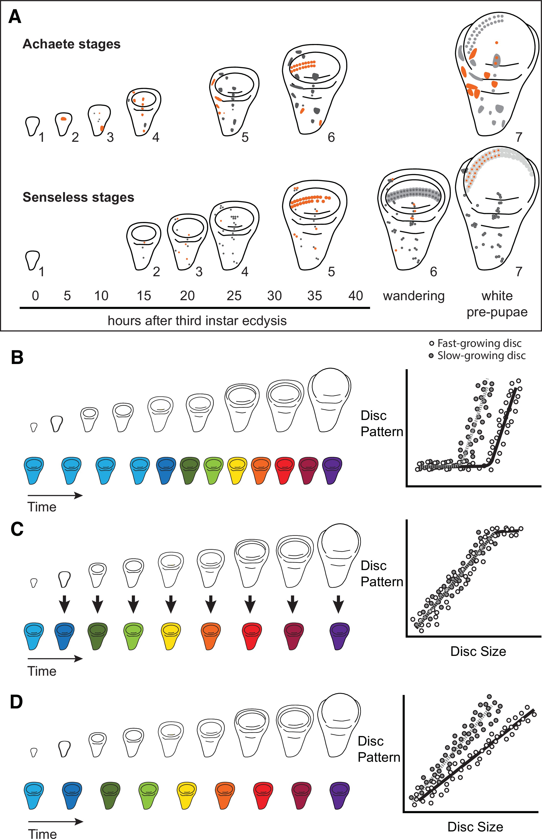
Characterizing organ growth rates is experimentally straightforward, requiring only accurate measurement of changes in organ size over time. To quantify the progression of organ patterning, however, requires developing a staging scheme. We previously developed such a scheme for the wing imaginal disc in D. melanogaster. This scheme makes use of the dynamic changes in expression from the moult to the third instar to pupariation of up to seven patterning-gene products in the developing wing 64Oliveira et al.2014. Two of these patterning-gene products, Achaete and Senseless, can be classed into seven different stages throughout third-instar development (64Oliveira et al.2014, Figure 1A), providing us with the ability to quantify the progression of wing disc pattern over a variety of conditions. In short, by describing patterning on a near-continuous scale, our scheme not only allows us to determine under what conditions patterning is initiated, but also the rate at which it progresses.

Quantitative assessments of the progression of patterning allow us to test hypotheses about the relationship between the size and patterning stage of the developing wing.

(A) The staging scheme developed by 64Oliveira et al.2014 to quantify the progression of Achaete and Senseless pattern. The pattern elements shown in orange are diagnostic for each stage, which is indicated by the number beside the disc. (**B–D**) The relationship between wing disc size and patterning stage (represented as wing discs progressing through a series of colours) if (B) Hypothesis 1: wing discs grow first and then initiate pattern; (C) Hypothesis 2: wing disc patterning is regulated by wing disc size (arrows); and (D) Hypothesis 3: wing disc pattern and growth are regulated at least partially independently.

The ability to simultaneously quantify both organ growth and pattern allows us to generate, and test, hypotheses regarding how ecdysone coordinates plastic growth with robust patterning. One hypothesis is that growth and patterning occur at different times, with ecdysone driving growth first then pattern later, or vice versa 53Mirth and Shingleton2019. If this were true, we would expect to identify an interval where ecdysone concentrations primarily affected growth and a second interval where they affected mostly pattern (Figure 1B). There is some precedence for this idea; most of the patterning in the wing discs and ovaries of D. melanogaster occurs 15 hr after the moult to the third larval instar 47Mendes and Mirth2016. Similarly, wing discs are known to grow faster in the early part of the third instar and slow their growth in the mid-to-late third instar 74Shingleton et al.2008. As a second hypothesis, ecdysone could coordinate plastic growth with robust pattern if the impacts of ecdysone on one of these processes depended on its effects on the other. For example, morphogens are known to regulate both growth and patterning of the wing. If ecdysone controlled the action of morphogens, we would expect the progression of patterning to be tightly coupled to growth over time, with different aspects of patterning being initiated at different disc sizes (Figure 1C). Finally, a third hypothesis is that ecdysone regulates the growth and patterning of the wing discs independently, and that each process responds in a qualitatively and quantitatively different manner to ecdysone 53Mirth and Shingleton2019. As an example of this, we might see that growth rates increase in a graded response to increasing ecdysone while patterning shows threshold responses, or vice versa. If this were the case, we would expect that growth and the progression of pattern would be uncoupled over time (Figure 1D).

Here, we test these hypotheses of whether and how ecdysone co-regulates plastic growth and robust pattern in wing imaginal discs in D. melanogaster. We blocked the production of ecdysone by genetically ablating the PG 36Herboso et al.2015 and quantified the effects on growth and patterning rates throughout the third instar. We then manipulated the rate of ecdysone synthesis by up- or down-regulating the activity of the insulin-signalling pathway in the PG 49Mirth et al.200541Koyama et al.2014 to test how this alters the relationship between disc size and disc pattern. Finally, we tested our hypotheses about how a single steroid can regulate both plastic growth and robust patterning by conducting dose-response experiments under two nutritional conditions. These studies provide a foundation for a broader understanding of how developmental hormones coordinate both plastic and robust responses across varying environmental conditions during animal development.

Results

Ecdysone is necessary for the progression of growth and patterning

To understand how ecdysone affects the dynamics of growth and patterning, we needed to be able to precisely manipulate ecdysone concentrations. For this reason, we made use of a technique we developed previously to genetically ablate the PGs (referred to as PGX) 36Herboso et al.2015. This technique pairs the temperature-sensitive repressor of GAL4, GAL80^ts, with a PG-specific GAL4 (phm-GAL4) to drive an apoptosis-inducing gene (UAS-GRIM). GAL80^ts is active at 17°C, where it represses GAL4 action, but inactive above 25°C, which allows phm-GAL4 to drive expression of UAS-GRIM and ablate the PG 45McGuire et al.200346McGuire et al.2004. Because ecdysone is required at every moult, we reared larvae from egg to the third larval instar (L3) at 17°C to repress GAL4, then shifted the larvae to 29°C at the moult to the third instar to generate PGX larvae.

PGX larvae had significantly reduced ecdysteroid titres than control genotypes (Figure 2—figure supplement 1). This method of reducing ecdysteroid concentration in the larvae allows us to examine how reducing ecdysone titres affects disc size and pattern in third-instar wing imaginal discs and manipulate ecdysone concentrations by adding it back in specific concentrations to the food 36Herboso et al.2015. For simplicity, all the data from the two control strains (either the phm-GAL4; GAL80ts or UAS-GRIM parental strain crossed to w¹¹¹⁸) were pooled in all analyses.

Insect wing discs show damped exponential, or fast-then-slow, growth dynamics 74Shingleton et al.200857Nijhout and Wheeler1996. These types of growth dynamics have frequently been modelled using a Gompertz function, which assumes that exponential growth rates slow down with time. The growth of wing discs from control and PGX larvae shows the same pattern, with a Gompertz function providing a significantly better fit to the relationship between log disc size and time than a linear function (ANOVA, linear vs. Gompertz model, n > 93, F > 65, p<0.001 for discs from both PGX and control larvae). Growth of the discs, however, followed a significantly different trajectory in PGX versus control larvae (Figure 2, Supplementary file 1a). In control larvae, discs continue to grow until 42 hr after ecdysis to the third instar (AEL3) when the larvae pupariate. In contrast, the wing imaginal discs of the PGX larvae grow at slower rates between 0 and 25 hr AEL3 (Figure 2, Supplementary file 1a) and stop growing at approximately 25 hr AEL3 at a significantly smaller size. This is despite the fact that PGX larvae do not pupariate, and so disc growth is not truncated by metamorphosis.

Figure 2.

#' @width 28
#' @height 20

# Packages
library("ggplot2")
library("lme4")
library("nlme")
library("deSolve")
library("MASS")
library("gdata")
library("gtools")
library("plyr")
library("dplyr")
library("nlstools")
library("tibble")
library("gridExtra")
library("grid")
library("car")
library("mosaic")
library("cowplot")
library("readr")
library("emmeans")
library("multcomp")
library("multcompView")
library("broom")
library("drc")

# Import data
PGXdata <- read_csv("PGXdata.csv", col_types = cols(X1 = col_skip()))
PGXrescue <- read_csv("PGXrescue.csv", col_types = cols(X1 = col_skip()))
PGX.starved <- read_csv("PGX.starved.csv", col_types = cols(X1 = col_skip()))
Pattern_Size<-read_csv("Pattern_Size.csv", col_types = cols(X1 = col_skip()))
PGX_E<-read_csv("PGX_E.csv", col_types = cols(X1 = col_skip()))
ecdysone.titres <- read_csv("EcdysoneQuantifications.csv", col_types = cols(X1 = col_skip()))


# We first explore how ablation of the PG affects growth and patterning of the wing imaginal discs. We will pool the control data, and remove Sens (Senseless) data since this is from the same disc as the Ac (Achaete) data.
dt <- PGXdata %>% filter(gene.product != "sens")  %>% mutate(Group = derivedFactor(
						"Control"=(genotype == "w_Grim" | genotype == "PG_w"),
						"Exp"=(genotype == "PGX"),
						.method="first"))

PGX.lm<-lm(logdisc.area~timepoint, data=subset(dt, genotype=="PGX"))
PGX.nls<- nls(logdisc.area ~ SSgompertz(timepoint, Asym, b2, b3), data=subset(dt, genotype=="PGX"))
#anova(PGX.nls,PGX.lm)
#coef(PGX.nls)
#confint2(PGX.nls)

control.lm<-lm(logdisc.area~timepoint, data=subset(dt, genotype=="w_Grim" |genotype=="PG_w" ))
control.nls<- nls(logdisc.area ~ SSgompertz(timepoint, Asym, b2, b3), data=subset(dt, genotype=="w_Grim"|genotype=="PG_w"))
#anova(control.nls,control.lm)
#coef(control.nls)
#confint2(control.nls)

PGX_all<- nls(logdisc.area ~ SSgompertz(timepoint, Asym, b2, b3), data=dt,start = list(Asym = rep(10, 1), b2 = rep(0.1, 1), b3 = rep(0.9, 1)))
#coef(PGX_all)

PGX_group<- nls(logdisc.area ~ SSgompertz(timepoint, Asym[Group], b2[Group], b3[Group]), data=dt,start = list(Asym = rep(10, 2), b2 = rep(0.1, 2), b3 = rep(0.9, 2)))
#coef(PGX_group)
#confint(PGX_group, level = 1-(0.05/1))
#anova(PGX_all,PGX_group)

#WHich Paramaters are Different?
PGX_group_dropAsym<- nls(logdisc.area ~ SSgompertz(timepoint, Asym, b2[Group], b3[Group]), data=dt,start = list(Asym = rep(10, 1), b2 = rep(0.1, 2), b3 = rep(0.9, 2)))

PGX_group_dropb2<- nls(logdisc.area ~ SSgompertz(timepoint, Asym[Group], b2, b3[Group]), data=dt,start = list(Asym = rep(10, 2), b2 = rep(0.1, 1), b3 = rep(0.9, 2)))

PGX_group_dropb3<- nls(logdisc.area ~ SSgompertz(timepoint, Asym[Group], b2[Group], b3), data=dt,start = list(Asym = rep(10, 2), b2 = rep(0.1, 2), b3 = rep(0.9, 1)))

#anova(PGX_group,PGX_group_dropAsym)
#anova(PGX_group,PGX_group_dropb2)
#anova(PGX_group,PGX_group_dropb3)

# Plot
ggplot(data=dt,aes(x=timepoint,y=logdisc.area, color = Group))+
  xlab("Time (hours after L3 moult)")+
ylab("ln Disc Size (nm2)")+
theme_bw()+
theme(panel.grid=element_blank(),axis.title.x=element_text(size=20), axis.title.y=element_text(size=20), 
        axis.text.y=element_text(size=16), axis.text.x=element_text(size=16), panel.background = element_rect(colour = "black"), legend.background = element_rect(), legend.key = element_rect(colour = "white"), legend.text=element_text(face="italic", size=16))+
 theme(legend.title=element_blank())+
 theme(axis.title.x = element_text(vjust=-0.5), axis.title.y = element_text(vjust=1.5))+
 scale_y_continuous(breaks = c(9, 9.5, 10, 10.5, 11, 11.5))+
geom_smooth(method = "nls", formula = y ~ SSgompertz(x, phi1, phi2, phi3), se = FALSE, size = 1)+
  geom_point(position = position_jitter(width = 0, height = 0.3), alpha = 0.5, size = 3)+
  #ggtitle("Figure 1")+
  #scale_color_brewer(palette = "Set2", labels = c("Control", "PGX"))
  scale_colour_manual(values=c("grey50", "#b2182b"), labels = c("Control", "PGX"))+
  scale_fill_manual(values=c("grey50", "#b2182b"), labels = c("Control", "PGX"))

Growth rates of wing discs are reduced in larvae with genetically ablated prothoracic glands (PGX) versus control larvae.

Curves are Gompertz functions of disc size against time (hours after the third larval instar (L3) moult). Parameters for the curves are significantly different between PGX and control (Supplementary file 1a). Control genotypes are the pooled results from both parental controls (either the phm-GAL4; GAL80ts, or UAS-GRIM parental strain crossed to w¹¹¹⁸). Each point represents the size of an individual wing disc. N_PGX = 95, N_Control = 125 across all time points.

Figure 2—figure supplement 1.

#' @width 28
#' @height 20
# Titrating Ecdysone

## Ecdysone in Food and Hemolymph
#First calculate ecdysone levels as pg per mg of larvae or as pg per larvae
ecdysone.titres <-ecdysone.titres %>% mutate(pg_mg_larvae = Ecdysone.concentration.real/weight, pg_L3 = Ecdysone.concentration.real/sample)

ecdysone.titres <- ecdysone.titres %>% mutate(Group = derivedFactor(
         "Control" = (genotype == "w_Grim" |  genotype == "PG_w"),
         "PGX" = (genotype == "PGX")))

#look at titres with 0 20E and fully fed

ecdysone.model.mg0<-lm(pg_L3 ~ Group, data= subset(ecdysone.titres, D20E == 0 & food == "Fed")) 
#Anova(ecdysone.model.mg0)
#summary(ecdysone.model.mg0)

means.20Ecompare <- emmeans(ecdysone.model.mg0, ~ Group)
#multcomp::cld(means.20Ecompare)

ggplot(data= subset(ecdysone.titres, D20E == 0 & food == "Fed"), aes(x= Group, y= pg_L3, colour = Group, fill = Group))+ 
xlab("Genotype")+
ylab("Ecdysteroid titre \n (pg/larva)")+
theme_bw()+
theme(panel.grid=element_blank(), axis.title.x=element_text(size=24), axis.title.y=element_text(size=24), axis.text.y=element_text(size=20), axis.text.x=element_text(size=20), panel.background = element_rect(colour = "black"), legend.title=element_blank(), legend.background = element_rect(), legend.key = element_rect(colour = "white"), legend.text=element_text(face="italic", size=24))+ 
 theme(axis.title.x = element_text(vjust=-0.5), axis.title.y = element_text(vjust=1.5))+theme(strip.text.x = element_text(size = 16))+
 #scale_y_continuous(limits=c(10,28))+
 #scale_x_continuous(limits=c(1.4,2.2))+
scale_colour_manual(values=c("grey50", "#b2182b"))+
scale_fill_manual(values=c("grey50", "#b2182b"))+
geom_point(size=5, alpha=0.7)+
geom_violin(alpha = 0.5) +
geom_blank()

Ecdysteroid titres in genetically ablated prothoracic glands (PGX) and control larvae.

Newly ecdysed larvae were placed on sucrose/yeast diets. Ecdysteroid titres in control (phm> + and + >grim) are significantly higher ecdysteroid titres than PGX larvae, as determined by linear models and pairwise comparisons of the means (F-value_{1, 13} = 10.75, p-value=0.006, N_control = 10, N_PGX = 5). Data is plotted with violin plots, and the individual replicates (five per genotype) are included as points overlaying the violin plots.

We next explored how the loss of ecdysone affected the progression of wing patterning. We used the staging scheme that we previously devised in 64Oliveira et al.2014 to quantify the progression of wing disc patterning in PGX and control larvae. We selected two gene-products from this scheme, Achaete and Senseless, as they each progress through seven stages throughout the third instar. Further we can stain for both antigens in the same discs, which allowed us to compare disc size, Achaete stage, and Senseless stage in the same sample.

The progression of Achaete patterning was best fit by a Gompertz function for discs from both PGX and control larvae (ANOVA, linear versus Gompertz model, n > 48, F > 10.4, p=0.002) 64Oliveira et al.2014 and was significantly affected by reduced ecdysone titres in PGX larvae. In control larvae, the wing discs progressed to Achaete stage 6 or 7 out of seven stages by 42 hr AEL3, while in PGX larvae, discs of the same age had not passed Achaete stage 3, and had not matured past Achaete stage 5 by 92 hr AEL3 (Figure 3A, Supplementary file 1b). The progression of Senseless patterning was best fit by a linear model, but again was significantly affected by reduced ecdysone titres. In control larvae, most discs had progressed to Senseless stage 6 out of seven stages by 42 hr AEL3, while no disc progressed past Senseless stage 2 by 92 hr AEL3 (Figure 3B, Supplementary file 1c).

Figure 3.

#' @width 28
#' @height 20
# Next we will look at how patterning of Achaete and Senseless is affected by ablation of the PG. We will look at Achaete patterning first, then Senseless patterning

dt <- PGXdata %>% filter(gene.product == "ac") %>% mutate(Group = derivedFactor(
						"Control"=(genotype == "w_Grim" | genotype == "PG_w"),
						"Exp"=(genotype == "PGX"),
						.method="first"))

Controlachaete.lm <- lm(gene.stage ~ timepoint, data = subset(dt, gene.product == "ac" & Group=="Control"))
Controlachaete.nls = nls(gene.stage ~ SSgompertz(timepoint, Asym, b2, b3), data = subset(dt, gene.product == "ac"& Group=="Control"))
#anova(Controlachaete.nls,Controlachaete.lm)

PGXachaete.lm <- lm(gene.stage ~ timepoint, data = subset(dt, gene.product == "ac" & Group=="Exp"))
PGXachaete.nls = nls(gene.stage ~ SSgompertz(timepoint, Asym, b2, b3), data = subset(dt, gene.product == "ac"& Group=="Exp"))
#anova(PGXachaete.nls,PGXachaete.lm)

# Now we can test whether the Gompertz curve is significantly different between control and PGX larvae.

PGXAchaete.nls_single = nls(gene.stage ~ SSgompertz(timepoint, Asym, b2, b3), data = dt)

PGXAchaete.nls_group = nls(gene.stage ~ SSgompertz(timepoint, Asym[Group], b2[Group], b3[Group]), data = dt, start = list(Asym = rep(8, 2), b2 = rep(2, 2), b3 = rep(0.97, 2)))

#anova(PGXAchaete.nls_single, PGXAchaete.nls_group)
#coef(PGXAchaete.nls_group)
#confint2(PGXAchaete.nls_group)



# Which Parameter is Different?

PGXAchaete_group_dropAsym<- nls(gene.stage ~ SSgompertz(timepoint, Asym, b2[Group], b3[Group]), data=dt,start = list(Asym = rep(4, 1), b2 = rep(1, 2), b3 = rep(0.9, 2)))

PGXAchaete_group_dropb2<- nls(gene.stage ~ SSgompertz(timepoint, Asym[Group], b2, b3[Group]), data=dt,start = list(Asym = rep(4, 2), b2 = rep(1, 1), b3 = rep(0.9, 2)))

PGXAchaete_group_dropb3<- nls(gene.stage ~ SSgompertz(timepoint, Asym[Group], b2[Group], b3), data=dt,start = list(Asym = rep(4, 2), b2 = rep(1, 2), b3 = rep(0.9, 1)))

#anova(PGXAchaete.nls_group,PGXAchaete_group_dropAsym)
#anova(PGXAchaete.nls_group,PGXAchaete_group_dropb2)
#anova(PGXAchaete.nls_group,PGXAchaete_group_dropb3)


# Now plotting the two curves, the difference is clear.

Figure_3A <- ggplot(data = dt, aes(x = timepoint, y = gene.stage, color = Group, fill = Group))+ 
xlab("Time (hours after L3 moult)")+
ylab("Achaete Stage")+
theme_bw()+
theme(panel.grid=element_blank(),axis.title.x=element_text(size=20), axis.title.y=element_text(size=20), 
        axis.text.y=element_text(size=16), axis.text.x=element_text(size=16), panel.background = element_rect(colour = "black"), legend.background = element_rect(), legend.key = element_rect(colour = "white"), legend.text=element_text(face="italic", size=16))+
 theme(legend.title=element_blank())+
 theme(axis.title.x = element_text(vjust=-0.5), axis.title.y = element_text(vjust=1.5))+
 scale_y_continuous(breaks = c(1, 2, 3, 4, 5, 6, 7))+
geom_smooth(method = "nls", formula = y ~ SSgompertz(x, phi1, phi2, phi3), se = FALSE, size = 1)+ 
  geom_point(position = position_jitter(width = 0, height = 0.3), alpha = 0.5, size = 3)+
#ggtitle("Figure 2A")+ 
#scale_color_brewer(palette = "Set2", labels = c("Control", "PGX"))
  scale_colour_manual(values=c("grey50", "#b2182b"), labels = c("Control", "PGX"))+
  scale_fill_manual(values=c("grey20", "#b2182b"), labels = c("Control", "PGX"))


# Now we will do the same for Senseless patterning, which is best fit with a linear function. Indeed a Gompertz function cant be fit for the PGX data.

dt <- PGXdata %>% filter(gene.product == "sens") %>% mutate(Group = derivedFactor(
						"Control"=(genotype == "w_Grim" | genotype == "PG_w"),
						"Exp"=(genotype == "PGX"),
						.method="first"))

PGXsens.lm<- lm(gene.stage ~ timepoint, data = subset(dt, Group == "Exp"))
#PGXsens.nls = nls(gene.stage ~ SSgompertz(timepoint, Asym, b2, b3), data = subset(dt, Group == "Exp"))

# Wont fit

Controlsens.lm<- lm(gene.stage ~ timepoint, data = subset(dt, Group == "Control"))
Controlsens.nls = nls(gene.stage ~ SSgompertz(timepoint, Asym, b2, b3), data = subset(dt, Group == "Control"))

#anova(Controlsens.nls,Controlsens.lm)

# We can fit a Gompertz function to the control data, and it provides a better fit, but to allow comparison between control and experimental we will use a linear function for both.

PGXSens.lm_group <- lm(gene.stage ~ timepoint * Group, data = dt)
#summary(PGXSens.lm_group)
#coef(PGXSens.lm_group)
#confint(PGXSens.lm_group)
#Anova(PGXSens.lm_group, type="III")

# Now we can plot the data
Figure_3B <- ggplot(data = dt, aes(x = timepoint, y = gene.stage, colour = Group, fill = Group))+ 
xlab("Time (hours after L3 moult)")+
ylab("Senseless Stage")+
theme_bw()+
theme(panel.grid=element_blank(),axis.title.x=element_text(size=20), axis.title.y=element_text(size=20), 
        axis.text.y=element_text(size=16), axis.text.x=element_text(size=16), panel.background = element_rect(colour = "black"), legend.background = element_rect(), legend.key = element_rect(colour = "white"), legend.text=element_text(face="italic", size=16))+
 theme(legend.title=element_blank())+
 theme(axis.title.x = element_text(vjust=-0.5), axis.title.y = element_text(vjust=1.5))+
 scale_y_continuous(breaks = c(1, 2, 3, 4, 5, 6, 7))+
  geom_point(position = position_jitter(width = 0, height = 0.3), alpha = 0.5, size = 3)+
geom_smooth(method = "lm", formula = y ~ x, se = FALSE, size = 1)+ 
#ggtitle("Figure 2B")+ 
#scale_color_brewer(palette = "Set2", labels = c("Control", "PGX"))
  scale_colour_manual(values=c("grey50", "#b2182b"), labels = c("Control", "PGX"))+
  scale_fill_manual(values=c("grey50", "#b2182b"), labels = c("Control", "PGX"))

# Plot 3A and B
Figure_3ANoL <- Figure_3A + theme(legend.position='none',axis.title.x=element_text(size=15), axis.title.y=element_text(size=15),axis.text.y=element_text(size=10), axis.text.x=element_text(size=10))
Figure_3BNoL <- Figure_3B + theme(legend.position='none',axis.title.x=element_text(size=15), axis.title.y=element_text(size=15),axis.text.y=element_text(size=10), axis.text.x=element_text(size=10))
legend <- get_legend(Figure_3A)
ggdraw(plot_grid(plot_grid(Figure_3ANoL, Figure_3BNoL, ncol=2, align='h'),
                 plot_grid(NULL, legend, ncol=1), rel_widths=c(1, 0.2))) +
  draw_plot_label(c("A", "B"), c(0, 0.41), c(1, 1), size = 20)

Achaete and Senseless patterning of wing discs is delayed in larvae with genetically ablated prothoracic glands (PGX) versus control larvae.

(A) Curves are Gompertz functions of Achaete stage against time (hours after the third instar (L3) moult). Parameters for the curves are significantly different between PGX and control (Supplementary file 1b). (B) Lines are linear regression of Senseless stage against time (hours after the L3 moult). Parameters for the lines are significantly different between PGX and control (Supplementary file 1c). Control genotypes are the pooled results from both parental controls (either the phm-GAL4; GAL80ts, or UAS-GRIM parental strain crossed to w¹¹¹⁸). For Achaete: N_PGX = 50, N_Control = 61, for Senseless: N_PGX = 52, N_Control = 54 across all time points.

We found no evidence of temporal separation between wing disc growth and the progression of pattern (compare Figures 2 and 3). Both growth and patterning progressed at steady rates throughout most of the third instar in control larvae, slowing down only at the later stages of development. Thus, the hypothesis that ecdysone coordinates plastic growth with robust pattern by acting on each process at different times (Figure 1B; Hypothesis 1) is not correct.

To confirm that reduced ecdysone titres were responsible for delayed patterning, and not a systemic response to the death of the glands, we performed a second experiment where we added either the active form of ecdysone, 20-hydroxyecdysone (20E), or ethanol (the carrier) back to the food. PGX and control larvae were transferred onto either 20E or ethanol food and allowed to feed for 42 hr, after which we dissected their wing discs and examined their size and pattern. On the control (ethanol) food, wing discs from PGX larvae were smaller (Figure 4A, Supplementary file 1d) and showed reduced patterning for both Achaete (Figure 4B, Supplementary file 1d) and Senseless (Figure 4C, Supplementary file 1d) when compared to control genotypes. Adding 0.15 mg of 20E/mg food fully restored disc size, and Achaete and Senseless pattern, such that they were indistinguishable from control genotypes fed on 20E-treated food.

Figure 4.

#' @width 28
#' @height 20
# To demonstrate that it is the lack of ecysone that is suppressing growth and patterning rather than a systemic repsonse to death of the PG, we can add ecdysone back in.

dt <- PGXrescue %>% mutate(Group = derivedFactor(
						"Control"=(genotype == "w_Grim" | genotype == "PG_w"),
						"Exp"=(genotype == "PGX"),
						.method="first"))


PGXrescueSize <- lm(logdisc.area ~  Group * medium, data = dt)
#summary(PGXrescueSize)
#Anova(PGXrescueSize)
emmeans.size <- emmeans(PGXrescueSize, ~ Group * medium)
#CLD(emmeans.size)

PGXrescueAchaete <- lm(Ac.stage ~  Group * medium, data = dt)
#summary(PGXrescueAchaete)
#Anova(PGXrescueAchaete)
emmeans.Achaete <- emmeans(PGXrescueAchaete, ~ Group * medium)
#CLD(emmeans.Achaete)

PGXrescueSens <- lm(Sens.stage ~  Group * medium, data = dt)
#summary(PGXrescueSens)
#Anova(PGXrescueSens)
emmeans.Sens <- emmeans(PGXrescueSens, ~ Group * medium)
#CLD(emmeans.Sens)

dt <- PGXrescue %>% mutate(Group = derivedFactor(
						"Control"=(genotype == "w_Grim" | genotype == "PG_w"),
						"PGX"=(genotype == "PGX"),
						.method="first"))


#dt$Group<-factor(dt$Group,level=c("Control", "Exp"))
dt$medium<-factor(dt$medium,level=c("ethanol", "20E"))

detach("package:plyr", unload = TRUE)

#THE FOLLOWING CODE WILL RETURN AN ERROR IF plyr IS ATTACHED DUE TO A CONFLICT BETWEEN plyr AND dplyr

labeldat = dt %>%
     group_by(Group, medium) %>%
     summarize(ypos = max(logdisc.area) + .1 ) %>% mutate(Group_med = paste(Group, medium, sep = "_") , sig_level = derivedFactor(
       "A" = ((Group == "Control" & medium  == "ethanol") | (Group == "PGX" & medium  == "20E")),
       "B" = (Group == "Control" & medium  == "20E"),
       "C" = (Group == "PGX" & medium  == "ethanol"),
						.method="first"))

Figure_4A<-ggplot(aes(y = logdisc.area, x = Group, fill = medium), data = dt) +
   geom_violin(aes(fill=medium), alpha = 0.5, position = position_dodge(width = 0.7)) +
  geom_point(aes(colour = medium),position=position_jitterdodge(jitter.width = 0.1, dodge=0.7), size=1)+
ylab("ln Disc Size (nm2)")+
xlab("")+
theme_bw()+
theme(panel.grid=element_blank(),axis.title.x=element_text(size=15), axis.title.y=element_text(size=15), 
        axis.text.y=element_text(size=10), axis.text.x=element_text(face="italic",size=15), panel.background = element_rect(colour = "black"), legend.background = element_rect(), legend.key = element_rect(colour = "white"), legend.text=element_text(size=15))+
 theme(legend.title=element_blank())+
 theme(axis.title.x = element_text(vjust=-0.5), axis.title.y = element_text(vjust=1.5))+ 
  coord_cartesian(ylim=c(9.5,12))+
#ggtitle("Figure 3A")+ 
 scale_colour_manual(values=c("grey50", "#1793bd"), labels = c("Ethanol", "Ecdysone"))+
  scale_fill_manual(values=c("grey50", "#1793bd"), labels = c("Ethanol", "Ecdysone"))+
  geom_text(data = labeldat, aes(label = sig_level, y = ypos), position = position_dodge(width = .7), show.legend = FALSE )


labeldat <- dt %>% 
     group_by(Group, medium) %>% summarise(ypos =  (max(Ac.stage) + 0.1)) %>%
      mutate(Group_med = paste(Group, medium, sep = "_") , sig_level = derivedFactor(
       "A" = ((Group == "Control" & medium  == "ethanol") | (Group == "Control" & medium  == "20E") | (Group == "PGX" & medium  == "20E")),
       "B" = (Group == "PGX" & medium  == "ethanol"),
						.method="first"))

Figure_4B<-ggplot(aes(y = Ac.stage, x = Group, fill = medium), data = dt)  +
   geom_violin(aes(fill=medium), alpha = 0.5, position = position_dodge(width = 0.7)) +
  geom_point(aes(colour = medium),position=position_jitterdodge(jitter.width = 0.1, dodge=0.7), size=1)+
ylab("Achaete Stage")+
xlab("")+
theme_bw()+
theme(panel.grid=element_blank(),axis.title.x=element_text(size=15), axis.title.y=element_text(size=15), 
        axis.text.y=element_text(size=10), axis.text.x=element_text(face="italic",size=15), panel.background = element_rect(colour = "black"), legend.background = element_rect(), legend.key = element_rect(colour = "white"), legend.text=element_text(size=15))+
 theme(legend.title=element_blank())+
 theme(axis.title.x = element_text(vjust=-0.5), axis.title.y = element_text(vjust=1.5))+ 
  coord_cartesian(ylim=c(0.5,7.5))+
   scale_y_continuous(breaks = c(1, 2, 3, 4, 5, 6, 7))+
#ggtitle("Figure 3B")+ 
 scale_colour_manual(values=c("grey50", "#1793bd"), labels = c("Ethanol", "Ecdysone"))+
  scale_fill_manual(values=c("grey50", "#1793bd"), labels = c("Ethanol", "Ecdysone"))+
  geom_text(data = labeldat, aes(label = sig_level, y = c(7.3, 7.3, 5.3, 7.3)), position = position_dodge(width = .7), show.legend = FALSE )


labeldat <- dt %>% 
     group_by(Group, medium) %>% summarise(ypos =  (max(Sens.stage) + 0.1)) %>%
      mutate(Group_med = paste(Group, medium, sep = "_") , sig_level = derivedFactor(
       "A" = (Group == "Control" & medium  == "ethanol"),
       "B" = ((Group == "Control" & medium  == "20E") | (Group == "PGX" & medium  == "20E")),
       "C" = (Group == "PGX" & medium  == "ethanol"),
						.method="first"))

Figure_4C<-ggplot(aes(y = Sens.stage, x = Group, fill = medium), data = dt)  +
   geom_violin(aes(fill=medium), alpha = 0.5, position = position_dodge(width = 0.7)) +
  geom_point(aes(colour = medium),position=position_jitterdodge(jitter.width = 0.1, dodge=0.7), size=1)+
ylab("Senseless Stage")+
xlab("")+
theme_bw()+
theme(panel.grid=element_blank(),axis.title.x=element_text(size=15), axis.title.y=element_text(size=15), 
        axis.text.y=element_text(size=10), axis.text.x=element_text(face="italic",size=15), panel.background = element_rect(colour = "black"), legend.background = element_rect(), legend.key = element_rect(colour = "white"), legend.text=element_text(size=15))+
 theme(legend.title=element_blank())+
 theme(axis.title.x = element_text(vjust=-0.5), axis.title.y = element_text(vjust=1.5))+
  coord_cartesian(ylim=c(0.5,7.5))+
   scale_y_continuous(breaks = c(1, 2, 3, 4, 5, 6, 7))+
#ggtitle("Figure 3C")+ 
 scale_colour_manual(values=c("grey50", "#1793bd"), labels = c("Ethanol", "Ecdysone"))+
  scale_fill_manual(values=c("grey50", "#1793bd"), labels = c("Ethanol", "Ecdysone"))+
  geom_text(data = labeldat, aes(label = sig_level, y = c(7.3, 7.3, 2.3, 7.3)), position = position_dodge(width = .7), show.legend = FALSE )

Figure_4ANoL <- Figure_4A + theme(legend.position='none')
Figure_4BNoL <- Figure_4B + theme(legend.position='none')
Figure_4CNoL <- Figure_4C + theme(legend.position='none')
legend <- get_legend(Figure_4A)
ggdraw() +
  draw_plot(Figure_4ANoL, 0.05, 0.5, 0.45, 0.5) +
  draw_plot(Figure_4BNoL, 0.05, 0, 0.45, 0.5) +
  draw_plot(Figure_4CNoL, 0.55, 0, 0.45, 0.5) +
  draw_plot(legend, 0.5, 0.5, 0.45, 0.5) +
  draw_plot_label(c("A", "B", "C"), c(0, 0, 0.5), c(1, 0.5, 0.5), size = 20)

Supplementing genetically ablated prothoracic gland (PGX) larvae with 20-hydroxyecdysone (20E) rescues wing disc growth (A), and Achaete (B) and Senseless (C) patterning.

Both the control and PGX larvae were exposed to 20E-treated food (0.15 mg/mg of food) or ethanol-treated food (which contains the same volume of ethanol) at 0 hr after the third instar moult. Wing discs were removed at 42 hr after the third instar moult. Control genotypes are the pooled results from both parental controls (either the phm-GAL4; GAL80ts, or UAS-GRIM parental strain crossed to w¹¹¹⁸). Treatments marked with different letters are significantly different (Tukey’s HSD, p<0.05, for ANOVA see Supplementary file 1d). Data were plotted using violin plots with individual wing discs displayed over the plots. N_{PGX + ethanol} = 21, N_{PGX + 20E} = 23, N_{Control +
ethanol} = 43, N_{Control + 20E} = 42.

Collectively, these data indicate that ecdysone is necessary for the normal progression of growth and patterning in wing imaginal discs. The loss of ecdysone has a more potent effect on patterning, however, which is effectively shutdown in PGX larvae, than on disc growth, which continues, albeit at a slower rate, for the first 24 hr of the third instar in PGX larvae.

Ecdysone rescues patterning and some growth in wing discs of yeast-starved larvae

The observation that ecdysone is necessary to drive both normal growth and patterning suggests that it may play a role in coordinating growth and patterning across environmental conditions. However, to do so it must lie downstream of the physiological mechanisms that sense and respond to environmental change. As discussed above, ecdysone synthesis is regulated by the activity of the insulin-signalling pathway, which is in turn regulated by nutrition. Starving larvae of yeast early in the third instar both suppress insulin signalling and inhibit growth and patterning of organs 50Mirth et al.200947Mendes and Mirth2016. We explored whether ecdysone was able to rescue some of this inhibition by transferring larvae immediately after the moult to 1% sucrose food that contained either 20E or ethanol and comparing their growth and patterning after 24 hr to wing discs from larvae fed on normal food. Both the PGX and control genotype failed to grow and pattern on the 1% sucrose with ethanol (Figure 5A–C, Supplementary file 1e). Adding 20E to the 1% sucrose food rescued Achaete and Senseless patterning in both the control and the PGX larvae to levels seen in fed controls (Figure 5B, Supplementary file 1e). 20E also partially rescued disc growth in PGX larvae, although not to the levels of the fed controls (Figure 5A). Collectively, these data suggest that the effect of nutrition on growth and patterning is at least partially mediated through ecdysone.

Figure 5.

#' @width 28
#' @height 20
dt <- PGX.starved %>% mutate(Group = derivedFactor(
						"Control"=(genotype == "w_Grim" | genotype == "PG_w"),
						"Exp"=(genotype == "PGX"),
						.method="first"))



PGXStarvedSize <- lm(logdisc.area ~  Group * medium, data = subset(dt, gene.product == "ac"))
#summary(PGXStarvedSize)
#Anova(PGXStarvedSize, type="III")
emmeans.size <- emmeans(PGXStarvedSize, ~ Group * medium)
#CLD(emmeans.size)

PGXStarvedAchaete <- lm(gene.stage ~  Group * medium, data = subset(dt, gene.product == "ac"))
#summary(PGXStarvedAchaete)
emmeans.Ac <- emmeans(PGXStarvedAchaete, ~ Group * medium)
#CLD(emmeans.Ac)

PGXStarvedSens <-lm(gene.stage ~  Group * medium, data = subset(dt, gene.product == "sens"))
#summary(PGXStarvedSens)
#Anova(PGXStarvedSens, type="III")
emmeans.Sens <- emmeans(PGXStarvedSens, ~ Group * medium)
#CLD(emmeans.Sens)

dt <- PGX.starved %>% mutate(Group = derivedFactor(
						"Control"=(genotype == "w_Grim" | genotype == "PG_w"),
						"PGX"=(genotype == "PGX"),
						.method="first"))



dtA<-subset(dt, gene.product=="ac")


 
labeldat = dtA %>%
     group_by(Group, medium) %>%
     summarize(ypos = max(logdisc.area) + .1 ) %>% mutate(Group_med = paste(Group, medium, sep = "_") , sig_level = derivedFactor(
       "A" = ((Group == "Control" & medium  == "1ethanol") | (Group == "PGX" & medium  == "1ethanol")),
       "B" = (Group == "Control" & medium  == "20E"),
       "C" = ((Group == "PGX" & medium  == "20E") | (Group == "PGX" & medium  == "normal.food")),
       "D" = (Group == "Control" & medium  == "normal.food"),
						.method="first"))

Figure_5A<-ggplot(aes(y = logdisc.area, x = Group, fill = medium), data = dtA)+
  geom_violin(aes(fill=medium), alpha = 0.5, position = position_dodge(width = 0.6)) +
  geom_point(aes(colour = medium),position=position_jitterdodge(jitter.width = 0.1, dodge=0.6), size=1)+
ylab("ln Disc Size (nm2)")+
xlab("")+
theme_bw()+
theme(panel.grid=element_blank(),axis.title.x=element_text(size=15), axis.title.y=element_text(size=15), 
        axis.text.y=element_text(size=10), axis.text.x=element_text(face="italic",size=15), panel.background = element_rect(colour = "black"), legend.background = element_rect(), legend.key = element_rect(colour = "white"), legend.text=element_text(size=15))+
 theme(legend.title=element_blank())+
 theme(axis.title.x = element_text(vjust=-0.5), axis.title.y = element_text(vjust=1.5))+ 
  coord_cartesian(ylim=c(8.5,11.5))+
#ggtitle("Figure 4A")+ 
scale_colour_manual(values=c("#a6e1f5", "#1793bd", "grey50"), labels = c("Starved + Ethanol", "Starved + Ecdysone", "Fed"))+
  scale_fill_manual(values=c("#a6e1f5", "#1793bd", "grey50"), labels = c("Starved + Ethanol", "Starved + Ecdysone", "Fed"))+
  geom_text(data = labeldat, aes(label = sig_level, y = ypos), position = position_dodge(width = .6), show.legend = FALSE )

labeldat <- dtA %>% 
     group_by(Group, medium) %>% summarise(ypos =  (max(gene.stage) + 0.2)) %>%
      mutate(Group_med = paste(Group, medium, sep = "_") , sig_level = derivedFactor(
       "A" = ((Group == "Control" & medium  == "1ethanol") | (Group == "PGX" & medium  == "1ethanol")),
       "B" = (Group == "PGX" & medium  == "normal.food"),
       "C" = (Group == "Control" & medium  == "20E"),
       "CD" = (Group == "Control" & medium  == "normal.food"),
       "D" = (Group == "PGX" & medium  == "20E"),
						.method="first"))

Figure_5B<-ggplot(aes(y = gene.stage, x = Group, fill = medium), data = dtA)   +
  geom_violin(aes(fill=medium), alpha = 0.5, position = position_dodge(width = 0.6)) +
  geom_point(aes(colour = medium),position=position_jitterdodge(jitter.width = 0.1, dodge=0.6), size=1)+
ylab("Achaete Stage")+
xlab("")+
theme_bw()+
theme(panel.grid=element_blank(),axis.title.x=element_text(size=15), axis.title.y=element_text(size=15), 
        axis.text.y=element_text(size=10), axis.text.x=element_text(face="italic",size=15), panel.background = element_rect(colour = "black"), legend.background = element_rect(), legend.key = element_rect(colour = "white"), legend.text=element_text(size=15))+
 theme(legend.title=element_blank())+
 theme(axis.title.x = element_text(vjust=-0.5), axis.title.y = element_text(vjust=1.5))+
  coord_cartesian(ylim=c(0.5,7))+
  scale_y_continuous(breaks = c(1, 2, 3, 4, 5, 6, 7))+
#ggtitle("Figure 4B")+ 
scale_colour_manual(values=c("#a6e1f5", "#1793bd", "grey50"), labels = c("Starved + Ethanol", "Starved + Ecdysone", "Fed"))+
  scale_fill_manual(values=c("#a6e1f5", "#1793bd", "grey50"), labels = c("Starved + Ethanol", "Starved + Ecdysone", "Fed"))+
  geom_text(data = labeldat, aes(label = sig_level, y = ypos), position = position_dodge(width = .6), show.legend = FALSE )

dtS<-subset(dt, gene.product=="sens")

labeldat <- dtS %>% 
     group_by(Group, medium) %>% summarise(ypos =  (max(gene.stage) + 0.2)) %>%
      mutate(Group_med = paste(Group, medium, sep = "_") , sig_level = derivedFactor(
       "A" = ((Group == "Control" & medium  == "1ethanol") | (Group == "PGX" & medium  == "1ethanol") | (Group == "PGX" & medium  == "normal.food")),
       "B" = (Group == "Control" & medium  == "20E"),
       "C" = (Group == "Control" & medium  == "normal.food") | (Group == "PGX" & medium  == "20E"),
						.method="first"))


Figure_5C<-ggplot(aes(y = gene.stage, x = Group, fill = medium), data = dtS)+
  geom_violin(aes(fill=medium), alpha = 0.5, position = position_dodge(width = 0.6)) +
  geom_point(aes(colour = medium),position=position_jitterdodge(jitter.width = 0.1, dodge=0.6), size=1)+
ylab("Senseless Stage")+
xlab("")+
theme_bw()+
theme(panel.grid=element_blank(),axis.title.x=element_text(size=15), axis.title.y=element_text(size=15), 
        axis.text.y=element_text(size=10), axis.text.x=element_text(face="italic",size=15), panel.background = element_rect(colour = "black"), legend.background = element_rect(), legend.key = element_rect(colour = "white"), legend.text=element_text(size=15))+
 theme(legend.title=element_blank())+
 theme(axis.title.x = element_text(vjust=-0.5), axis.title.y = element_text(vjust=1.5))+
  coord_cartesian(ylim=c(0.5,6))+
 coord_cartesian(ylim=c(0.5,7))+
  scale_y_continuous(breaks = c(1, 2, 3, 4, 5, 6, 7))+
#ggtitle("Figure 4B")+ 
scale_colour_manual(values=c("#a6e1f5", "#1793bd", "grey50"), labels = c("Starved\n+ Ethanol", "Starved\n+ Ecdysone", "Fed"))+
  scale_fill_manual(values=c("#a6e1f5", "#1793bd", "grey50"), labels = c("Starved\n+ Ethanol", "Starved\n+ Ecdysone", "Fed"))+
  geom_text(data = labeldat, aes(label = sig_level, y = ypos), position = position_dodge(width = .6), show.legend = FALSE )

Figure_5ANoL <- Figure_5A + theme(legend.position='none')
Figure_5BNoL <- Figure_5B + theme(legend.position='none')
Figure_5CNoL <- Figure_5C + theme(legend.position='none')
legend <- get_legend(Figure_5A)
ggdraw() +
  draw_plot(Figure_5ANoL, 0.05, 0.5, 0.45, 0.5) +
  draw_plot(Figure_5BNoL, 0.05, 0, 0.45, 0.5) +
  draw_plot(Figure_5CNoL, 0.55, 0, 0.45, 0.5) +
  draw_plot(legend, 0.5, 0.5, 0.45, 0.5) +
  draw_plot_label(c("A", "B", "C"), c(0, 0, 0.5), c(1, 0.5, 0.5), size = 20)

Supplementing genetically ablated prothoracic gland (PGX) larvae with 20-hydroxyecdysone (20E) is able to partially rescue the effect of yeast starvation on (A) wing discs growth, and fully rescue (B) Achaete and (C) Senseless patterning.

Both the control and PGX larvae were exposed from 0 hr after the third instar moult to one of three food types: (1) starved + 20 E – starvation medium containing 1% sucrose and 1% agar laced with 20E (0.15 mg/mg of food), (2) starved + ethanol – starvation medium treated with the same volume of ethanol, or (3) fed – normal fly food. Wing discs were removed at 24 hr after the third instar moult. Control genotypes are the pooled results from both parental controls (the UAS-GRIM parental strain crossed to w¹¹¹⁸). Treatments marked with different letters are significantly different (Tukey’s HSD, p<0.05, for ANOVA see Supplementary file 1e). Data were plotted using violin plots with individual wing discs displayed over the plots. N_{PGX + starved -
ethanol} = 23, N_{PGX + starved - 20E} = 22, N_{PGX + fed} = 26, N_{Control +
starved-ethanol} = 28, N_{Control + starved-20E} = 22, N_{Control + fed} = 27.

An important aspect of these data is that in PGX larvae either supplementing the 1% sucrose food with 20E or feeding them on normal food both rescued wing disc growth (Figure 5A), albeit incompletely. This suggests that nutrition can drive growth through mechanisms independent of ecdysone, and vice versa. In contrast, nutrition alone only marginally promoted Achaete and Senseless patterning in starved PGX larvae, while 20E alone completely restored patterning. Further, even early patterning did not progress in PGX larvae (Figure 3). Thus, the effect of nutrition on patterning appears to be wholly mediated by ecdysone, while the effect of nutrition on growth appears to be partially mediated by ecdysone and partially through another independent mechanism. Ecdysone-independent growth appears to occur early in the third larval instar, however, since disc growth in PGX and control larvae is more or less the same in the first 12 hr after ecdysis to L3 (Figure 2).

Ecdysone drives growth and patterning independently

The data above suggest a model of growth and patterning, where both ecdysone and nutrition can drive growth, but where patterning is driven by ecdysone. We next focused on exploring how ecdysone regulates both growth and patterning. Patterning genes, particularly morphogens, are known to regulate growth, so one hypothesis is that ecdysone promotes patterning, which in turn promotes the ecdysone-driven component of disc growth. A second related hypothesis is that ecdysone-driven growth is necessary to promote patterning. Under either of these hypotheses, because the mechanisms regulating patterning and growth are interdependent, we would expect that changes in ecdysone levels would not change the relationship between disc size and disc pattern. An alternative hypothesis, therefore, is that ecdysone promotes growth and patterning through at least partially independent mechanisms. Under this hypothesis, the relationship between size and patterning may change at different levels of ecdysone.

To distinguish between these two hypotheses, we increased or decreased the activity of the insulin-signalling pathway in the PG, which is known to increase or decrease the level of circulating ecdysone, respectively 7Caldwell et al.200541Koyama et al.201415Colombani et al.200549Mirth et al.2005. We then looked at how these manipulations affected the relationship between disc size and disc pattern, again focusing on Achaete and Senseless patterning. We increased insulin signalling in the PG by overexpressing InR (phm>InR) and reduced insulin signalling by overexpressing the negative regulator of insulin signalling PTEN (P0206>PTEN).

We found that a linear model is sufficient to capture the relationship between disc size and Achaete stage when we either increase (phm>InR: AIC_linear – AIC_logistic = 22, ANOVA, F_(25,27) = 1.71, p=0.2018) or decrease ecdysone synthesis rates (P0206>PTEN). Changing ecdysone levels, however, significantly changed the parameters of the linear model and altered the relationship between disc size and Achaete pattern. Specifically, increasing ecdysone level shifted the relationship so that later stages of Achaete patterning occurred in smaller discs (Figure 6A, Supplementary file 1f).

Figure 6.

#' @width 28
#' @height 20
# Relationship Between Size and Pattern
# We first need to set up the data tables

dt <- Pattern_Size %>% filter(gene.product == "Ac" |gene.product == "Sens") %>% mutate(umdata = 1000000 * disc.area, logdisc.area = log(umdata))

dt<- dt %>% filter(genotype == "phm.InR" | genotype == "InRcontrol"|genotype == "P0206.PTEN" | genotype == "PTENcontrol")

dt <- dt%>% mutate(Group = derivedFactor(
						"phm.InR"=(genotype == "phm.InR"),
						"Control"=(genotype == "InRcontrol"| genotype == "PTENcontrol"),
						"P0206.PTEN"=(genotype == "P0206.PTEN"),
						.method="first"))

dt$genotype<-drop.levels(dt$genotype)

## Senseless
### Stats
# We first to test whether a threshold or linear function is the best fit for the data. The threshold function is a 4 parameter logistic. The parameterization we are using is A+(B-A)/(1+exp((xmid-input)/scal)), where A is minimum, B is maximum, xmid is the inflection point and scal is (1/scal), where scal is the logistic growth rate, or the steepness of the curve.

##all data
Allsens.rate <- lm(gene.stage ~ logdisc.area, data = subset(dt, gene.product == "Sens"))
Allsens.threshold <-  nls(gene.stage ~ SSfpl(logdisc.area, A,B,xmid,scal), data = subset(dt, gene.product == "Sens"))
#anova(Allsens.threshold, Allsens.rate)
#AIC(Allsens.threshold, Allsens.rate)

##InR Control
InRcontrolsens.rate <- lm(gene.stage ~ logdisc.area, data = subset(dt, gene.product == "Sens" & genotype == "InRcontrol"))
InRcontrolsens.threshold <-  nls(gene.stage ~ SSfpl(logdisc.area, A,B,xmid,scal), data = subset(dt, gene.product == "Sens" & genotype == "InRcontrol"))
#anova(InRcontrolsens.threshold, InRcontrolsens.rate)
#AIC(InRcontrolsens.threshold, InRcontrolsens.rate)

##phm>InR
phmInRsens.rate <- lm(gene.stage ~ logdisc.area, data = subset(dt, gene.product == "Sens" & genotype == "phm.InR"))

phmInRsens.threshold <-  nls(gene.stage ~ SSfpl(logdisc.area, A,B,xmid,scal), data = subset(dt, gene.product == "Sens" & genotype == "phm.InR"))

#anova(phmInRsens.threshold, phmInRsens.rate)
#AIC(phmInRsens.threshold, phmInRsens.rate)

##PTEN Control
PTENcontrolsens.rate  <- lm(gene.stage ~ logdisc.area, data = subset(dt, gene.product == "Sens" & genotype == "PTENcontrol"))

PTENcontrolsens.threshold <-  nls(gene.stage ~ SSfpl(logdisc.area, A,B,xmid,scal), data = subset(dt, gene.product == "Sens" & genotype == "PTENcontrol"))

#anova(PTENcontrolsens.threshold, PTENcontrolsens.rate)
#AIC(PTENcontrolsens.threshold, PTENcontrolsens.rate)

##P0206>PTEN
P0206PTENsens.rate  <- lm(gene.stage ~ logdisc.area, data = subset(dt, gene.product == "Sens" & genotype == "P0206.PTEN"))


P0206PTENsens.threshold <-  nls(gene.stage ~ SSfpl(logdisc.area, A,B,xmid,scal), data = subset(dt, gene.product == "Sens" & genotype == "P0206.PTEN"))


#anova(P0206PTENsens.threshold, P0206PTENsens.rate)
#AIC(P0206PTENsens.threshold, P0206PTENsens.rate)

#Senseless is best fit with a threshold function.

#Now we can test whether the parameters of the model change with changes in ecdysone.
#(For the parameters, 1 = phm.InR, 2 = Control, 3 = P0206.PTEN)

# Is there a difference between groups across all parameters?
Sens.threshold_single <-  nls(gene.stage ~ SSfpl(logdisc.area, A,B,xmid,scal), data = subset(dt, gene.product == "Sens"),  start = list(A = rep(0.9, 1), B = rep(8, 1), xmid = rep(11, 1), scal=rep(0.5, 1)))
#summary(Sens.threshold_single)

model.drm3 <- drm (gene.stage ~ logdisc.area, data = subset(dt, gene.product == "Sens"), fct = LL.4())

Sens.threshold_group <-  nls(gene.stage ~ SSfpl(logdisc.area, A[Group],B[Group],xmid[Group],scal[Group]), data = subset(dt, gene.product == "Sens"),  start = list(A = rep(1, 3), B = rep(7, 3), xmid = rep(11, 3), scal=rep(0.3, 3)))
#coef(Sens.threshold_group)
#confint2(Sens.threshold_group, level=(1-(0.05/3)))

#anova(Sens.threshold_group,Sens.threshold_single)

#Which parameter?

Sens.threshold_groupdropA <-  nls(gene.stage ~ SSfpl(logdisc.area, A,B[Group],xmid[Group],scal[Group]), data = subset(dt, gene.product == "Sens"),  start = list(A = rep(1, 1), B = rep(7, 3), xmid = rep(11, 3), scal=rep(0.3, 3)))

Sens.threshold_groupdropB <-  nls(gene.stage ~ SSfpl(logdisc.area, A[Group],B,xmid[Group],scal[Group]), data = subset(dt, gene.product == "Sens"),  start = list(A = rep(1, 3), B = rep(7, 1), xmid = rep(11, 3), scal=rep(0.3, 3)))

Sens.threshold_groupdropxmid <-  nls(gene.stage ~ SSfpl(logdisc.area, A[Group],B[Group],xmid,scal[Group]), data = subset(dt, gene.product == "Sens"),  start = list(A = rep(1, 3), B = rep(7, 3), xmid = rep(11, 1), scal=rep(0.3, 3)))

Sens.threshold_groupdropscal <-  nls(gene.stage ~ SSfpl(logdisc.area, A[Group],B[Group],xmid[Group],scal), data = subset(dt, gene.product == "Sens"),  start = list(A = rep(1, 3), B = rep(7,3), xmid = rep(11, 3), scal=rep(0.3, 1)))

#anova(Sens.threshold_group,Sens.threshold_groupdropA)
#anova(Sens.threshold_group,Sens.threshold_groupdropB)
#anova(Sens.threshold_group,Sens.threshold_groupdropxmid)
#anova(Sens.threshold_group,Sens.threshold_groupdropscal)

Figure_6B <- ggplot(data = subset(dt, gene.product == "Sens"), aes(x = logdisc.area, y = gene.stage, colour = Group, fill = Group))+ 
xlab("ln Disc Size (nm2)")+
ylab("Senseless Stage")+
theme_bw()+
theme(panel.grid=element_blank(),axis.title.x=element_text(size=15), axis.title.y=element_text(size=15), 
        axis.text.y=element_text(size=10), axis.text.x=element_text(size=10), panel.background = element_rect(colour = "black"), legend.background = element_rect(), legend.key = element_rect(colour = "white"), legend.text=element_text(face="italic", size=16))+
theme(legend.title=element_blank())+
 theme(axis.title.x = element_text(vjust=-0.5), axis.title.y = element_text(vjust=1.5))+
   scale_y_continuous(limits = c(1,7.5),breaks = c(1, 2, 3, 4, 5, 6, 7))+
  scale_x_continuous(breaks = c(8, 9, 10, 11, 12))+
geom_point(size = 3, shape = 16, alpha = 0.5)+ 
  geom_smooth(method = "nls", formula = y ~ SSfpl(x, A, B, xmid, scal), se = FALSE, size = 1)+
#ggtitle("Figure 5A")+ 
#scale_color_brewer(palette = "Set2")
scale_colour_manual(values=c("#1793bd", "grey50", "#f0853e"), labels = c("phm>InR", "Control", "P0206>PTEN"))+
  scale_fill_manual(values=c("#1793bd", "grey50", "#f0853e"), labels = c("phm>InR", "Control", "P0206>PTEN"))

## Achaete
### Stats

#Now do the same with Achaete:
##all data
Allac.rate <- lm(gene.stage ~ logdisc.area, data = subset(dt, gene.product == "Ac"))
Allac.threshold <-  nls(gene.stage ~ SSfpl(logdisc.area, A,B,xmid,scal), data = subset(dt, gene.product == "Ac"))
#anova(Allac.threshold, Allac.rate)
#AIC(Allac.threshold, Allac.rate)

##InR Control
InRcontrolachaete.rate <- lm(gene.stage ~ logdisc.area, data = subset(dt, gene.product == "Ac" & genotype == "InRcontrol"))


InRcontrolachaete.threshold <-  nls(gene.stage ~ SSfpl(logdisc.area, A,B,xmid,scal), data = subset(dt, gene.product == "Ac" & genotype == "InRcontrol"))


#anova(InRcontrolachaete.threshold, InRcontrolachaete.rate)
#AIC(InRcontrolachaete.threshold, InRcontrolachaete.rate)

##phm>InR
phmInRachaete.rate <- lm(gene.stage ~ logdisc.area, data = subset(dt, gene.product == "Ac" & genotype == "phm.InR"))


phmInRachaete.threshold <-  nls(gene.stage ~ SSfpl(logdisc.area, A,B,xmid,scal), data = subset(dt, gene.product == "Ac" & genotype == "phm.InR"))

#anova(phmInRachaete.threshold, phmInRachaete.rate)
#AIC(phmInRachaete.threshold, phmInRachaete.rate)


##PTEN Control
PTENcontrolachaete.rate  <- lm(gene.stage ~ logdisc.area, data = subset(dt, gene.product == "Ac" & genotype == "PTENcontrol"))


PTENcontrolachaete.threshold <-  nls(gene.stage ~ SSfpl(logdisc.area, A,B,xmid,scal), data = subset(dt, gene.product == "Ac" & genotype == "PTENcontrol"))


#anova(PTENcontrolachaete.threshold, PTENcontrolachaete.rate)
#AIC(PTENcontrolachaete.threshold, PTENcontrolachaete.rate)

##P0206>PTEN
P0206PTENachaete.rate  <- lm(gene.stage ~ logdisc.area, data = subset(dt, gene.product == "Ac" & genotype == "P0206.PTEN"))

#P0206PTENachaete.threshold <-  nls(gene.stage ~ SSfpl(logdisc.area, A,B,xmid,scal), data = subset(dt, gene.product == "Ac" & genotype == "P0206.PTEN"),start = list(A = rep(0.2, 1), B = rep(8, 1), xmid = rep(11, 1), scal=rep(0.8, 1)))

#Won't resolve

#So the linear fit is better for the experimental flies but the threshold is better for the controls. In order to compare we need to use a linear fit.

### test for differences between genotypes

AchaeteLinear<-lm(gene.stage ~ Group*logdisc.area, data = subset(dt, gene.product == "Ac"))
#Anova(AchaeteLinear, type="III")
#coef(AchaeteLinear)
#confint(AchaeteLinear, level=(1-0.05/2))


# Test for pairwise differences
phmInRvC<-lm(gene.stage ~ logdisc.area + Group, data = subset(dt, gene.product == "Ac" & Group!="P0206.PTEN"))
#Anova(AchaeteLinear, type="II")

P0206.PTENRvC<-lm(gene.stage ~ logdisc.area*Group, data = subset(dt, gene.product == "Ac" & Group!="phm.InR"))
#Anova(AchaeteLinear, type="II")

#So there is a difference between genotype, but not between control and phm>InR

Figure_6A <-  ggplot(data = subset(dt, gene.product == "Ac"), aes(x = logdisc.area, y = gene.stage, colour = Group, fill = Group))+ 
xlab("ln Disc Size (nm2)")+
ylab("Achaete Stage")+
theme_bw()+
theme(panel.grid=element_blank(),axis.title.x=element_text(size=15), axis.title.y=element_text(size=15), 
        axis.text.y=element_text(size=10), axis.text.x=element_text(size=10), panel.background = element_rect(colour = "black"), legend.background = element_rect(), legend.key = element_rect(colour = "white"), legend.text=element_text(face="italic", size=16))+
theme(legend.title=element_blank())+
 theme(axis.title.x = element_text(vjust=-0.5), axis.title.y = element_text(vjust=1.5))+
    scale_y_continuous(limits = c(1,7.5),breaks = c(1, 2, 3, 4, 5, 6, 7))+
  scale_x_continuous(breaks = c(8, 9, 10, 11, 12))+
  geom_point(size = 3, shape = 16, alpha = 0.5)+
geom_smooth(method = "lm", formula = y ~ x, se = FALSE, size = 1)+
#ggtitle("Figure 5B")+ 
scale_colour_manual(values=c("#1793bd", "grey50", "#f0853e"), labels = c("phm>InR", "Control", "P0206>PTEN"))+
  scale_fill_manual(values=c("#1793bd", "grey50", "#f0853e"), labels = c("phm>InR", "Control", "P0206>PTEN"))

Figure_6ANoL <- Figure_6A + theme(legend.position='none')
Figure_6BNoL <- Figure_6B + theme(legend.position='none')
legend <- get_legend(Figure_6B)

ggdraw(plot_grid(plot_grid(Figure_6ANoL, Figure_6BNoL,ncol=2, align='v'),
                 plot_grid(NULL, legend, ncol=1), rel_widths=c(1, 0.3))) +
  draw_plot_label(c("A", "B"), c(0, 0.39), c(1, 1), size = 20)

Changing rate of ecdysteroid synthesis changes the relationship between disc pattern and disc size throughout the third-instar larval stage.

(A) The relationship between Achaete stage and disc size was fitted with a linear regression, the parameters of which are significantly different between genotypes (Supplementary file 1f). (B) The relationship between Senseless stage and disc size was fitted with a four-parameter logistic regression, the parameters of which are significantly different between genotypes (Supplementary file 1g). We staged third instar larvae from the onset of the moult to the formation of white prepupae. The length of this developmental interval varied across genotypes. For control genotypes, we sampled larvae at 0, 10, 20, 30, 48, and 51 (InR control)/53 (PTEN control) hr after third instar ecdysis (AL3E). For phm>InR, we sampled larvae at 0, 10, 20, 29, 30, and 36 hr AL3E. For P0206>PTEN, we sampled larvae at 0, 10, 20, 30, 40, 60, 73, and 80 hr AL3E. The number of discs sampled for each genotype and patterning gene was: for Achaete: N_phm>InR = 29, N_Control = 99, N_P0206>PTEN = 40, for Senseless: N_phm>InR = 29, N_Control = 99, N_P0206>PTEN = 41.

The relationship between Senseless pattern and disc size is best fit using a four-parameter logistic (threshold) function, which provides a significantly better fit to the data than a linear function (AIC_linear – AIC_logistic = 32.2; ANOVA, F_(44,46) = 25.8, p<0.001). Changing ecdysone levels significantly changed the parameters of the logistic model and altered the relationship between disc size and Senseless pattern (Figure 6B, Supplementary file 1g). Again, increasing ecdysone level shifted the relationship so that later stages of Senseless patterning occurred in smaller discs. Collectively, these data support the hypothesis that ecdysone acts on growth and patterning at least partially independently (Figure 1D; Hypothesis 3), and that patterning is not regulated by wing disc size (Figure 1C; Hypothesis 2).

Ecdysone regulates disc growth and disc patterning through different mechanisms

The data above support a model whereby environmental signals act through ecdysone to co-regulate growth and patterning, generating organs of variable size but invariable pattern. Further, growth is also regulated by an ecdysone-independent mechanism, enabling similar progressions of pattern across discs of different sizes. An added nuance, however, is that ecdysone levels are not constant throughout development. Rather, the ecdysone titre fluctuates through a series of peaks throughout the third larval instar and the dynamics of these fluctuations are environmentally sensitive 83Warren et al.2006. To gain further insight into how ecdysone co-regulates plasticity and robustness, we therefore explored which aspects of ecdysone dynamics regulate growth and patterning.

Two characteristics of ecdysone fluctuations appear to be important with respect to growth and patterning. First, the timing of the ecdysone peaks set the pace of development, initiating key developmental transitions such as larval wandering and pupariation 41Koyama et al.201449Mirth et al.200583Warren et al.200671Riddiford et al.1993. Second, the basal levels of ecdysone appear to regulate the rate of body growth, with an increase in basal level leading to a reduction in body growth 7Caldwell et al.200536Herboso et al.201515Colombani et al.200549Mirth et al.200552Mirth et al.2014. While several studies, including this one, have established that disc growth is positively regulated by ecdysone 36Herboso et al.201525Dye et al.201766Parker and Shingleton2011, whether disc growth is driven by basal levels or peaks of ecdysone is unknown.

There are a number of hypotheses as to how ecdysone levels may drive patterning and growth. One hypothesis is that patterning and ecdysone-regulated disc growth show threshold responses, which are initiated once ecdysone rises above a certain level. This would manifest as low patterning and growth rates when ecdysteroid titres were sub-threshold, and a sharp, switch-like increase in patterning and growth rates after threshold ecdysone concentrations was reached. Alternatively, both may show a graded response, with patterning and growth rates increasing continuously with increasing ecdysteroid titres. Finally, disc patterning may show one type of response to ecdysone, while disc growth may show another. Separating these hypotheses requires the ability to titrate levels of ecdysone.

To do this, we reared PGX larvae on standard food supplemented with a range of 20E concentrations (0, 6.25, 12.5, 25, 50, and 100 ng of ecdysone/mg of food). However, as noted above, disc growth early in the third larval instar is only moderately affected by ablation of the PG, potentially obfuscating the effects of supplemental 20Esupplemental 20ESupplementary file 1E. In contrast, discs from starved PGX larvae show no growth or patterning without supplemental 20E.supplemental 20E Supplementary file 1E We therefore also reared PGX larvae either on standard food or on 20% sucrose/1% agar medium (from hereon referred to as ‘starved’ larvae) supplemented with a range of 20E concentrations. For both control genotypes and PGX larvae, increasing the concentration of 20E in the food increased ecdysteroids titres in the larvae (Figure 7—figure supplement 1, Supplementary file 1h).

To quantify the effects of 20E concentration in the wing disc growth, we dissected discs at 5 hr intervals starting immediately after the moult to the third instar (0 hr AL3E) to 20 hr AL3E. Because male and female larvae show differences in wing disc growth 80Testa et al.2013, we separated the sexes in this experiment and focused our analysis on female wing discs.

As before, in both PGX and control larvae, wing disc growth was suppressed by starvation (Figure 7—figure supplement 2, Supplementary file 1i). To explore how disc size changed over time with increasing 20E concentration, we modelled the data using a second-order polynomial regression against time after third instar ecdysis. Increasing the concentration of supplemental 20E Supplementary file 1Eincreased the disc growth rate in starved PGX larvae (Figure 7A, Supplementary file 1j). In contrast, increasing 20E concentrations had no effect on disc growth rate in fed PGX larvae (Figure 7—figure supplement 3, Supplementary file 1j). This confirms that the effect of nutrition on growth masks the effect of 20E early in the third larval instar and supports that hypothesis that disc growth during this period is primarily regulated by nutrition and only moderately regulated by ecdysone 74Shingleton et al.2008.

Figure 7.

#' @width 28
#' @height 15
## Growth with Ecdysone
### Stats

growth.starvedLM <- lm(ln.disc.area ~ poly(timepoint, 2, raw = FALSE) * d20Ecat, data = dt)
#Anova(growth.starvedLM, Type = "III")
growth.trends <- emtrends(growth.starvedLM, ~ d20Ecat, var = "timepoint", max.degree = 1)
# multcomp::cld(growth.trends)

coefs.growthstarved <- tidy(growth.trends)
coefs.growthstarved$d20Ecat<-as.numeric(as.character(coefs.growthstarved$d20Ecat))
names(coefs.growthstarved)[1]<-"d20E"

dt<-PGX_E[PGX_E$genotype=="PGX" & PGX_E$food=="fed",]
# Anova(lm(ln.disc.area~d20E*poly(timepoint, degree=2), data=dt), type="III")

# Starved

Figure_7A<-ggplot(data=subset(PGX_E, genotype=="PGX" & food=="starved"), aes(x=timepoint,y=ln.disc.area, color=d20Ecat))+
   ylim(9.5,10.6)+
    xlab("Time (hours after L3 moult)")+
 ylab("ln Disc Size (nm2)")+
   ggtitle("Starved - PGX")+
   geom_smooth(method="lm",formula=y~poly(x, degree=2),se=F)+
   geom_point(size = 5, shape = 16, alpha = 0.5)+
   theme_bw()+
 theme(panel.grid=element_blank(),axis.title.x=element_text(size=15), axis.title.y=element_text(size=15),
         axis.text.y=element_text(size=16), axis.text.x=element_text(size=16), panel.background = element_rect(colour = "black"), legend.background = element_rect(), legend.key = element_rect(colour = "white"), legend.text=element_text(face="italic", size=16))+
 theme(legend.title=element_blank())+
  theme(axis.title.x = element_text(vjust=-0.5), axis.title.y = element_text(vjust=1.5))+
   scale_colour_brewer(type='seq', palette='RdGy', labels = c("0 - A","6.25 - AB","12.5 - ABC","25 - ABC","50 - C","100 - BC"))

# extract coefficients from emtrends
model.drm1 <- drm (timepoint.trend ~ d20E, data = coefs.growthstarved, fct = MM.3())
model.drm2 <- drm (timepoint.trend ~ d20E, data = coefs.growthstarved, fct = LL.3())
model.drm3 <- drm (timepoint.trend ~ d20E, data = coefs.growthstarved, fct = LL.4())

#AIC(model.drm1, model.drm2, model.drm3)
#BIC(model.drm1, model.drm2, model.drm3)


###Michaelis Menten is the best fit
mml <- data.frame(d20E = seq(0, max(coefs.growthstarved$d20E), length.out = 100))
mml$linear_growth <- predict(model.drm1, newdata = mml)


 Figure_7B<-ggplot(data=coefs.growthstarved, aes(x=d20E,y=timepoint.trend))+
    xlab("20E Concentration in Food (ng/ml)")+
 ylab("Disc linear growth rate")+
   scale_y_continuous(limits = c(0.02, 0.06), breaks = c(0.02, 0.03, 0.04, 0.05, 0.06))+
   ggtitle("Starved - PGX")+
   geom_line(data = mml, aes(x = d20E, y = linear_growth), colour = "black", size = 2)+
   geom_point(size = 5, shape = 16)+
   theme_bw()+
 theme(panel.grid=element_blank(),axis.title.x=element_text(size=15), axis.title.y=element_text(size=15), 
         axis.text.y=element_text(size=16), axis.text.x=element_text(size=16), panel.background = element_rect(colour = "black"), legend.background = element_rect(), legend.key = element_rect(colour = "white"), legend.text=element_text(face="italic", size=16))+
 theme(legend.title=element_blank())+
  theme(axis.title.x = element_text(vjust=-0.5), axis.title.y = element_text(vjust=1.5))
 
 ggdraw() +
   draw_plot(Figure_7A, 0, 0, 0.66, 1) +
   draw_plot(Figure_7B, 0.66, 0, 0.33, 1) +
   draw_plot_label(c("A", "B"), c(0, 0.65), c(1, 1), size = 20)

Effect of supplemental 20-hydroxyecdysone (20E) Supplementary file 1Eon growth of the wing imaginal disc in starved genetically ablated prothoracic gland (PGX) larvae.

Growth was modelled as S = E + T + T²+ E * T + E * T², where S = disc size, E = 20E concentration, and T = disc age. (A) There was a significant effect of E on the linear growth rate of the wing imaginal discs (Supplementary file 1j). Each point corresponds to a wing disc, N_{PGX – starved} = 409 (63–72 discs were sampled per treatment across all time points). 20E treatments that do not share a letter (see legend) are significantly different in patterning rates as determined by post-hoc test on the slopes (Supplementary file 1j). (B) The linear growth rate of the wing disc was extracted from the growth model for each concentration of 20E and modelled using a three-parameter Michaelis–Menten equation: y = c + (d-c)/(_1 + (b/x)), where _c is y at x = 0, d = y[max], and b is x where y is halfway between c and d. Linear growth rate increases steadily with ecdysone concentration in the food up until 25 ng of 20E/ml of food, after which growth rate increases more slowly with increasing 20E concentration.

Figure 7—figure supplement 1.

#' @width 28
#' @height 20
ggplot(data= ecdysone.titres, aes(x= D20E, y= pg_L3, colour = food, fill = food, shape = food, linetype = food))+ 
xlab("20E Concentration in Food (ng/ml)")+
ylab("Ecdysteroid titre \n (pg/larva)")+
theme_bw()+
theme(panel.grid=element_blank(), axis.title.x=element_text(size=24), axis.title.y=element_text(size=24), axis.text.y=element_text(size=20), axis.text.x=element_text(size=20), panel.background = element_rect(colour = "black"), legend.title=element_blank(), legend.background = element_rect(), legend.key = element_rect(colour = "white"), legend.text=element_text(face="italic", size=24))+ 
 theme(axis.title.x = element_text(vjust=-0.5), axis.title.y = element_text(vjust=1.5))+theme(strip.text.x = element_text(size = 16))+
 #scale_y_continuous(limits=c(10,28))+
 #scale_x_continuous(limits=c(1.4,2.2))+
scale_colour_manual(values=c("#4a4534", "#a19670"), labels = c("fed", "starved"))+
scale_fill_manual(values=c("#4a4534", "#a19670"), labels = c("fed", "starved"))+
geom_point(size=5, alpha=0.7)+
  scale_shape_manual(values=c(16, 1), labels = c("fed", "starved"))+
  scale_linetype_manual(values = c(1,2), labels = c("fed", "starved"))+
geom_smooth(method="lm", formula = y ~ poly(x, 2, raw=TRUE), se=FALSE, size = 1) +
facet_grid(. ~ Group)+
geom_blank()

The effects of 20-hydroxyecdysone (20E) concentration in the food on ecdysteroid titres in control and genetically ablated prothoracic gland (PGX) larvae.

Newly ecdysed larvae were placed on sucrose/yeast (fed) or 20% sucrose/1% agar (starved) diets supplemented with a range of 20E concentrations for 20 hr. They were then transferred to the same diet without 20E and dyed with blue food colouring for 2 hr to eliminate residual 20E in the gut. Ecdysteroid titres in fed and starved control (phm> + and + >grim) and PGX larvae fed a range of 20E concentrations. There is a significant positive relationship between 20E concentration in the food and the concentration of ecdysteroids in the larvae, as indicated by a significant 20E term (Supplementary file 1h). Furthermore, starved larvae had higher ecdysone titres than fed larvae. Open and closed points represent the biological replicates, and solid and dashed lines are linear regressions. N_{control - starved} = 60, N_{control - fed} = 60, N_{PGX - starved} = 30, N_{PGX - fed} = 30 across all 20E concentrations.

Figure 7—figure supplement 2.

#' @width 28
#' @height 20
## Growth w/o Ecdysone or Food
### Stats

#First we will test how ecdysone affects growth in discs from fed and starved PGX larvae without ecdysone. Quadratic function are best fit for growth across genotypes in fed conditions:

PGX_E <- PGX_E %>% mutate(Group = derivedFactor(
						"Control"=(genotype == "w_Grim" | genotype == "PG_w"),
						"Exp"=(genotype == "PGX"),
						.method="first"))
PGX_E$d20Ecat<-as.factor(PGX_E$d20Ecat)
PGX_E$food<-as.factor(PGX_E$food)

dt<-subset(PGX_E, food=="fed" & d20E==0 )

PGX.lm<-lm(ln.disc.area~timepoint, data=subset(dt, Group=="Exp"))
PGX.poly<-lm(ln.disc.area~poly(timepoint, 2), data=subset(dt, genotype=="PGX"))
PGX.nls<- nls(ln.disc.area ~ SSgompertz(timepoint, Asym, b2, b3), data=subset(dt, genotype=="PGX"))
#anova(PGX.nls,PGX.poly,PGX.lm)
#coef(PGX.poly)
#confint2(PGX.poly)
#summary(PGX.poly)

Control.lm<-lm(ln.disc.area~timepoint, data=subset(dt, Group=="Control"))
Control.poly<-lm(ln.disc.area~poly(timepoint, 2), data=subset(dt, Group=="Control"))
#Control.nls<- nls(ln.disc.area ~ SSgompertz(timepoint, Asym, b2, b3), data=subset(dt, Group=="Control"))
#anova(Control.poly,Control.lm)
#coef(Control.poly)
#confint2(Control.poly)
#summary(Control.poly)

#Across genotypes, growth is suppressed in starvation conditions.

dt<-subset(PGX_E, d20E==0 )
#Anova(lm<-lm(ln.disc.area~Group*food*poly(timepoint, degree=2), data=dt), type="III")

#There is a difference in starvation-response among genotypes.
dt<-subset(PGX_E, d20E==0 & food=="fed" )
#Anova(lm<-lm(ln.disc.area~Group*poly(timepoint, degree=2), data=dt), type="III")
#summary(lm(ln.disc.area~Group*poly(timepoint, degree=2), data=dt))[[4]]
#confint(lm(ln.disc.area~Group*poly(timepoint, degree=2), data=dt))

Sup_Figure_2A<-ggplot(data=subset(PGX_E, Group=="Exp" & d20Ecat =="0"), aes(x=timepoint,y=ln.disc.area, colour = food, fill = food, linetype = food))+
  ylim(9.5,10.75)+
   xlab("Time (hours after L3 moult)")+
ylab("ln Disc Size (nm2)")+
  geom_smooth(method="lm",formula=y~poly(x,2),se=F)+
  geom_point(aes(shape = food), size = 3, alpha = 0.5)+
   ggtitle("PGX")+ 
  theme_bw()+
theme(panel.grid=element_blank(),axis.title.x=element_text(size=15), axis.title.y=element_text(size=15), 
        axis.text.y=element_text(size=10), axis.text.x=element_text(size=10), panel.background = element_rect(colour = "black"), legend.background = element_rect(), legend.key = element_rect(colour = "white"), legend.text=element_text(face="italic", size=16))+
theme(legend.title=element_blank())+
 theme(axis.title.x = element_text(vjust=-0.5), axis.title.y = element_text(vjust=1.5))+
  scale_shape_manual(values=c(16, 1), labels = c("fed", "starved"))+
  scale_linetype_manual(values = c(1,2), labels = c("fed", "starved"))+
  scale_colour_manual(values=c("#b2182b", "#FF6600"))+
scale_fill_manual(values=c("#b2182b", "#FF6600"))


Sup_Figure_2B<-ggplot(data=subset(PGX_E, Group=="Control" & d20Ecat=="0"), aes(x=timepoint,y=ln.disc.area, colour = food, fill = food, linetype = food, shape = food))+
  ylim(9.5,10.75)+
   xlab("Time (hours after L3 moult)")+
ylab("ln Disc Size (nm2)")+
  geom_smooth(method="lm",formula=y~poly(x,2),se=F)+
  geom_point(aes(shape = food), size = 3, alpha = 0.5)+
   ggtitle("Control")+ 
  theme_bw()+
theme(panel.grid=element_blank(),axis.title.x=element_text(size=15), axis.title.y=element_text(size=15), 
        axis.text.y=element_text(size=10), axis.text.x=element_text(size=10), panel.background = element_rect(colour = "black"), legend.background = element_rect(), legend.key = element_rect(colour = "white"), legend.text=element_text(face="italic", size=16))+
theme(legend.title=element_blank())+
 theme(axis.title.x = element_text(vjust=-0.5), axis.title.y = element_text(vjust=1.5))+
  scale_shape_manual(values=c(16, 1), labels = c("fed", "starved"))+
  scale_linetype_manual(values = c(1,2), labels = c("fed", "starved"))+
  scale_colour_manual(values=c("#4a4534", "#a19670"))+
scale_fill_manual(values=c("#4a4534", "#a19670"))


ggdraw(plot_grid(plot_grid(Sup_Figure_2A, Sup_Figure_2B,ncol=2, align='v'))) +
  draw_plot_label(c("A", "B"), c(0, 0.5), c(1, 1), size = 20)

Wing imaginal disc growth is suppressed in fed genetically ablated prothoracic gland (PGX) larvae relative to controls and in starved larvae of both genotypes.

PGX (A) and control (B) larvae reared on sucrose/yeast (fed) or 20% sucrose/1% agar (starved) diets without 20E supplementation. Wing discs were sampled at 5 h intervals between 0-20 h after the moult to third instar. Wing disc growth was modelled as a quadratic, and there was a significant interaction between genotype (PGX vs. Control) and nutrition (fed vs. starved) on growth (Supplementary file 1i). Solid line/closed point = fed larvae, broken line/open point = starved larvae. Each point corresponds to a wing disc, N_{PGX - starved} = 67, N_{PGX - fed} = 74, N_{control -
starved} = 118, N_{control - fed} = 151 across all time points.

Figure 7—figure supplement 3.

#' @width 28
#' @height 20
ggplot(data=subset(PGX_E, genotype=="PGX" & food=="fed"), aes(x=timepoint,y=ln.disc.area, color=d20Ecat))+
  ylim(9.5,10.75)+
   xlab("Time (hours after L3 moult)")+
ylab("ln Disc Size (nm2)")+
  geom_smooth(method="lm",formula=y~poly(x, degree=2),se=F)+
  geom_point(size = 5, shape = 16, alpha = 0.5)+
  theme_bw()+
theme(panel.grid=element_blank(),axis.title.x=element_text(size=15), axis.title.y=element_text(size=15), 
        axis.text.y=element_text(size=16), axis.text.x=element_text(size=16), panel.background = element_rect(colour = "black"), legend.background = element_rect(), legend.key = element_rect(colour = "white"), legend.text=element_text(face="italic", size=16))+
theme(legend.title=element_blank())+
 theme(axis.title.x = element_text(vjust=-0.5), axis.title.y = element_text(vjust=1.5))+
  scale_colour_brewer(type='seq', palette='RdGy')

There is no effect of supplemental 20-hydroxyecdysone (20E) Supplementary file 1Eon growth of the wing imaginal disc in fed genetically ablated prothoracic gland (PGX) larvae.

Growth was modelled as S = E + T + T²+ E * T + E * T², where S = disc size, E = 20E concentration, and T = disc age. There was no significant effect of E on the linear or quadratic growth rate of the wing imaginal discs (Supplementary file 1j). Each point corresponds to a wing disc, N_{PGX – fed} = 459 (73–86 discs were sampled per treatment across all time points).

To test whether wing disc growth rates show either a graded or threshold response to 20E concentration in starved PGX larvae, we extracted the linear growth rate coefficients from our models. We then modelled the relationship between growth rate and 20E concentration with three nonlinear functions: a graded Michaelis–Menten function, and threshold three- and four-parameter log-logistic functions. Finally, we tested which model best fit the data using Akaike information criteria (AIC) and Bayesian information criteria (BIC) for model selection. The model with the lowest AIC and BIC values best fits the data.

When wing disc growth rate was modelled with the graded Michaelis–Menten function, both the AIC and BIC values were lower than when it was modelled with either threshold function (Supplementary file 1k). This supports the hypothesis that growth rate increases continuously with increasing 20E concentration, with growth rate plateauing after 20E concentrations reach 25 ng/ml (Figure 7B). Thus, disc growth rate appears to show a graded response to 20E level in the absence of nutrition. This is in line with recent ﬁndings from 77Strassburger et al.2021, which show that proliferation and growth in the wing discs increase with increasing 20E concentration in the diet 77Strassburger et al.2021.

The effect of 20E concentration on Achaete patterning was qualitatively different to its effect on growth. As before, Achaete patterning did not progress in either starved or fed PGX larvae (Figure 8—figure supplement 1). In contrast, Achaete patterning did progress in PGX larvae supplemented with 20E. Patterning rates for Achaete did not differ significantly between 0–6.25 ng/ml (fed) and 0–12.5 ng/ml (starved) of 20E (Figure 8A and C, Supplementary file 1). Above 25 ng/ml of 20E, Achaete patterning occurred at the same rapid rate in both fed and starved PGX larvae (Figure 8A and C).

Figure 8.

#' @width 28
#' @height 20
## Achaete Patterning with Ecdysone
#### Fed

dt<-subset(PGX_E, food=="fed" & genotype=="PGX")

ac.fedLM <- lm(ac.stage ~ poly(timepoint, 2, raw = FALSE) * d20Ecat, data = dt)
#Anova(ac.fedLM, type = "III")
ac.fed.trends <- emtrends(ac.fedLM, ~ d20Ecat, var = "timepoint", max.degree = 1)
#multcomp::cld(ac.fed.trends)

coefs.acfed <- tidy(ac.fed.trends)
coefs.acfed$d20Ecat<-as.numeric(as.character(coefs.acfed$d20Ecat))
names(coefs.acfed)[1]<-"d20E"

Figure_8A<-ggplot(data=subset(PGX_E, genotype=="PGX" & food=="fed"), aes(x=timepoint,y=ac.stage, color=d20Ecat))+
  scale_y_continuous(limits = c(0.5, 7.5), breaks = c(1, 2, 3, 4, 5, 6, 7))+
  xlab("Time (hours after L3 moult)")+
ylab("Achaete Stage")+
ggtitle("Fed - PGX")+
  scale_size(breaks = c(1, 5, 10, 20))+
  geom_smooth(method="lm",formula=y~poly(x, degree=2),se=F)+
  geom_count(position = position_jitter(width = 0.3, height = 0.3),shape=16, alpha=0.7)+
  theme_bw()+
theme(panel.grid=element_blank(),axis.title.x=element_text(size=15), axis.title.y=element_text(size=15), 
        axis.text.y=element_text(size=16), axis.text.x=element_text(size=16), panel.background = element_rect(colour = "black"), legend.background = element_rect(), legend.key = element_rect(colour = "white"), legend.text=element_text(face="italic", size=16))+
theme(legend.title=element_blank())+
 theme(axis.title.x = element_text(vjust=-0.5), axis.title.y = element_text(vjust=1.5))+
  scale_colour_brewer(type='seq', palette='RdGy', labels = c("0 - A","6.25 - A","12.5 - B","25 - BC","50 - BC","100 - C"))

# extract coefficients from emtrends

#which model fits best?

#from emtrends
model.drm1 <- drm (timepoint.trend ~ d20E, data = coefs.acfed, fct = MM.3())
model.drm2 <- drm (timepoint.trend ~ d20E, data = coefs.acfed, fct = LL.3())
model.drm3 <- drm (timepoint.trend ~ d20E, data = coefs.acfed, fct = LL.4())

#AIC(model.drm1, model.drm2, model.drm3)
#BIC(model.drm1, model.drm2, model.drm3)


mml <- data.frame(d20E = seq(0, max(coefs.acfed$d20E), length.out = 100))
mml$timepoint.trend <- predict(model.drm3, newdata = mml)

Figure_8B<-ggplot(data=coefs.acfed, aes(x=d20E,y=timepoint.trend))+
   xlab("20E Concentration in Food (ng/ml)")+
ylab("Achate patterning rate")+
  ggtitle("Fed - PGX")+
 scale_y_continuous(limits = c(0, 0.25), breaks = c(0, 0.05, 0.1, 0.15, 0.2, 0.25))+
  geom_line(data = mml, aes(x = d20E, y = timepoint.trend), colour = "black", size = 2)+
  geom_point(size = 5, shape = 16)+
  theme_bw()+
theme(panel.grid=element_blank(),axis.title.x=element_text(size=15), axis.title.y=element_text(size=15), 
        axis.text.y=element_text(size=16), axis.text.x=element_text(size=16), panel.background = element_rect(colour = "black"), legend.background = element_rect(), legend.key = element_rect(colour = "white"), legend.text=element_text(face="italic", size=16))+
theme(legend.title=element_blank())+
 theme(axis.title.x = element_text(vjust=-0.5), axis.title.y = element_text(vjust=1.5))

#Starved

dt<-subset(PGX_E, food=="starved" & genotype=="PGX")

ac.starvedLM <- lm(ac.stage ~ poly(timepoint, 2, raw = FALSE) * d20Ecat, data = dt)
#Anova(ac.starvedLM, type = "III")
ac.starved.trends <- emtrends(ac.starvedLM, ~ d20Ecat, var = "timepoint", max.degree = 1)
#multcomp::cld(ac.starved.trends)


coefs.acstarved <- tidy(ac.starved.trends)
coefs.acstarved$d20Ecat<-as.numeric(as.character(coefs.acstarved$d20Ecat))
names(coefs.acstarved)[1]<-"d20E"

Figure_8C<-ggplot(data=subset(PGX_E, genotype=="PGX" & food=="starved"), aes(x=timepoint,y=ac.stage, color=d20Ecat))+
  scale_y_continuous(limits = c(0.5, 7.5), breaks = c(1, 2, 3, 4, 5, 6, 7))+
  xlab("Time (hours after L3 moult)")+
ylab("Achaete Stage")+
  ggtitle("Starved - PGX")+
  scale_size(breaks = c(1, 5, 10, 20))+
  geom_smooth(method="lm",formula=y~poly(x, degree=2),se=F)+
  geom_count(position = position_jitter(width = 0.3, height = 0.3),shape=16, alpha=0.7)+
  theme_bw()+
theme(panel.grid=element_blank(),axis.title.x=element_text(size=15), axis.title.y=element_text(size=15), 
        axis.text.y=element_text(size=16), axis.text.x=element_text(size=16), panel.background = element_rect(colour = "black"), legend.background = element_rect(), legend.key = element_rect(colour = "white"), legend.text=element_text(face="italic", size=16))+
theme(legend.title=element_blank())+
 theme(axis.title.x = element_text(vjust=-0.5), axis.title.y = element_text(vjust=1.5))+
  scale_colour_brewer(type='seq', palette='RdGy', labels = c("0 - A","6.25 - A","12.5 - A","25 - B","50 - B","100 - B"))

# extract coefficients from emtrends

model.drm1 <- drm (timepoint.trend ~ d20E, data = coefs.acstarved, fct = MM.3())
model.drm2 <- drm (timepoint.trend ~ d20E, data = coefs.acstarved, fct = LL.3())
model.drm3 <- drm (timepoint.trend ~ d20E, data = coefs.acstarved, fct = LL.4())

#AIC(model.drm1, model.drm2, model.drm3)
#BIC(model.drm1, model.drm2, model.drm3)


mml <- data.frame(d20E = seq(0, max(coefs.acstarved$d20E), length.out = 100))
mml$timepoint.trend <- predict(model.drm3, newdata = mml)


Figure_8D<-ggplot(data=coefs.acstarved, aes(x=d20E,y=timepoint.trend))+
   xlab("20E Concentration in Food (ng/ml)")+
ylab("Achate patterning rate")+
  ggtitle("Starved - PGX")+
  scale_y_continuous(limits = c(0, 0.25), breaks = c(0, 0.05, 0.1, 0.15, 0.2, 0.25))+
  geom_line(data = mml, aes(x = d20E, y = timepoint.trend), colour = "black", size = 2)+
  geom_point(size = 5, shape = 16)+
  theme_bw()+
theme(panel.grid=element_blank(),axis.title.x=element_text(size=15), axis.title.y=element_text(size=15), 
        axis.text.y=element_text(size=16), axis.text.x=element_text(size=16), panel.background = element_rect(colour = "black"), legend.background = element_rect(), legend.key = element_rect(colour = "white"), legend.text=element_text(face="italic", size=16))+
theme(legend.title=element_blank())+
 theme(axis.title.x = element_text(vjust=-0.5), axis.title.y = element_text(vjust=1.5))

ggdraw() +
  draw_plot(Figure_8A, 0, 0.5, 0.66, .5) +
  draw_plot(Figure_8B, 0.66, 0.5, 0.33, .5) +
  draw_plot(Figure_8C, 0, 0, 0.66, .5) +
  draw_plot(Figure_8D, 0.66, 0, 0.33, .5) +
  draw_plot_label(c("A", "B", "C", "D"), c(0, 0.65, 0, 0.65), c(1, 1, 0.5, 0.5), size = 20)

Effect of supplemental 20-hydroxyecdysone (20E) Supplementary file 1Eon Achaete patterning of the wing imaginal disc in (A, B) fed and (C, D) starved genetically ablated prothoracic gland (PGX) larvae.

In (A) and (C), patterning stage was modelled as A = E + T + T²+ E * T + E * T², where A = Achaete stage, E = 20E concentration, and T = disc age. The size of each point corresponds to the number of wing disc in each stage. 20E treatments that do not share a letter (see legend) are significantly different in patterning rates as determined by post-hoc test on the slopes (for ANOVA, see Supplementary file 1l). In (B) and (D), we extracted the linear patterning rate from fed (B) or starved (D) PGX larvae. We then modelled the relationship between patterning rate and 20E concentration using a four-parameter log-logistic equation: y = c + (d)(–c)/(1 + e^{(b(log(x))-log(a))}), where c is the lower asymptote, d is the upper asymptote, b is the rate of increase, and a is the inflection point. N_{PGX – fed} = 459, N_{PGX – starved} = 409, 63–86 discs were sampled per treatment across all time points.

Figure 8—figure supplement 1.

#' @width 28
#' @height 13
## Achaete Patterning w/o Ecdysone or Food
### Stats
#The quadratic fit is probably the best overall. Using this model, we can test the effect of starvation on pattern development, and test whether it is affected by genotype.

dt<-PGX_E[PGX_E$d20E==0,]
#Anova(lm(ac.stage~food*Group*poly(timepoint, degree=2), data=dt), type="III")

# Test within PGX and Control
dt<-subset(PGX_E, Group=="Exp" & d20E==0)
#Anova(lm(ac.stage~food*poly(timepoint, degree=2), data=dt), type="III")

dt<-subset(PGX_E, Group=="Control" & d20E==0)
#Anova(lm(ac.stage~food*poly(timepoint, degree=2), data=dt), type="III")

Sup_Figure_4A<- ggplot(aes(y = ac.stage, x = timepoint, colour = food, fill = food, linetype = food), data = subset(PGX_E, Group=="Exp" & d20E=="0" ))+
  scale_y_continuous(limits = c(1, 7.5), breaks = c(1, 2, 3, 4, 5, 6, 7))+
  xlab("Time (hours after L3 moult)")+
ylab("Achaete Stage")+
   ggtitle("PGX")+
  geom_smooth(method = "lm", formula = y ~ poly(x, degree=2), se=F, aes(color=food))+
  geom_point(aes(shape=food),position = position_jitter(width = 0.3, height = 0.3),size = 3, alpha = 0.7)+ 
  theme_bw()+
theme(panel.grid=element_blank(),axis.title.x=element_text(size=15), axis.title.y=element_text(size=15), 
        axis.text.y=element_text(size=16), axis.text.x=element_text(size=16), panel.background = element_rect(colour = "black"), legend.background = element_rect(), legend.key = element_rect(colour = "white"), legend.text=element_text(face="italic", size=16))+
theme(legend.title=element_blank())+
 theme(axis.title.x = element_text(vjust=-0.5), axis.title.y = element_text(vjust=1.5))+
  scale_shape_manual(values=c(16, 1), labels = c("fed", "starved"))+
  scale_linetype_manual(values = c(1,2), labels = c("fed", "starved"))+
 scale_colour_manual(values=c("#b2182b", "#ef8a62"))+
scale_fill_manual(values=c("#b2182b", "#ef8a62"))
  


Sup_Figure_4B<- ggplot(aes(y = ac.stage, x = timepoint, color=food, fill = food, linetype = food), data = subset(PGX_E, Group=="Control" & d20E=="0" ))+
  ylim(1,6)+
  scale_y_continuous(limits = c(1, 7.5), breaks = c(1, 2, 3, 4, 5, 6, 7))+
  xlab("Time (hours after L3 moult)")+
ylab("Achaete Stage")+
  ggtitle("Control")+
  geom_smooth(method = "lm", formula = y ~ poly(x, degree=2), se=F, aes(color=food))+
  #geom_count(aes(color=food),position = position_jitter(width = 0.3, height = 0.3),shape=19)+
  geom_point(aes(shape = food),position = position_jitter(width = 0.3, height = 0.3),size = 3, alpha = 0.7)+ 
theme_bw()+
theme(panel.grid=element_blank(),axis.title.x=element_text(size=15), axis.title.y=element_text(size=15), 
        axis.text.y=element_text(size=16), axis.text.x=element_text(size=16), panel.background = element_rect(colour = "black"), legend.background = element_rect(), legend.key = element_rect(colour = "white"), legend.text=element_text(face="italic", size=16))+
theme(legend.title=element_blank())+
 theme(axis.title.x = element_text(vjust=-0.5), axis.title.y = element_text(vjust=1.5))+
  scale_shape_manual(values=c(16, 1), labels = c("fed", "starved"))+
  scale_linetype_manual(values = c(1,2), labels = c("fed", "starved"))+
scale_colour_manual(values=c("#4a4534", "#a19670"))+
scale_fill_manual(values=c("#4a4534", "#a19670"))

ggdraw(plot_grid(plot_grid(Sup_Figure_4A, Sup_Figure_4B,ncol=2, align='v'))) +
  draw_plot_label(c("A", "B"), c(0, 0.5), c(1, 1), size = 20)

Achaete patterning in wing discs from fed and starved genetically ablated prothoracic gland (PGX) and control larvae.

(A) Patterning does not progress in either fed or starved PGX larvae. (B) Patterning does not progress in starved control larvae but does in fed control larvae. There is a significant interaction between the effects of disc age and food on Achaete patterning in control larvae (orthogonal polynomial regression: $F_{{f o o d * d i s c a g e}^{2}}$ = 67.98, p<0.001), but not in PGX larvae (orthogonal polynomial regression: $F_{{f o o d * d i s c a g e}^{2}}$ = 1.81, p=0.163). Each point corresponds to a wing disc, N_{PGX - starved} = 67, N_{PGX - fed} = 74, N_{control -
starved} = 118, N_{control - fed} = 151 across all time points.

To compare the progression of Achaete at different levels of 20E with the progression of disc growth, we modelled the relationship between Achaete pattern, time after third-instar ecdysis, and 20E concentration as second-order polynomial regression for fed and starved PGX larvae. As for disc growth, we then extracted the linear coefficients from this model at each level of 20E and modelled the relationship between patterning rate and 20E using a Michaelis–Menten function and a three- and four-parameter log-logistic function. Both the AIC and BIC indicated that that a threshold four-parameter log-logistic function fit the data better than a graded Michaelis–Menten function (Supplementary file 1k). Thus, unlike growth, Achaete patterning showed a threshold response to 20E concentration. Specifically, Achaete patterning was not initiated unless 20E is above a certain concentration (12.5–25 ng/ml), but it progressed at the same rate regardless of how high 20E is above this concentration.

Comparing the timing of Achaete patterning in 20E-supplemented PGX larvae versus fed controls provides some indication of when in normal development the threshold level of 20E necessary to initiate Achaete patterning is reached. Discs from fed control larvae began to reach Achaete stage 4 by 15 hr AEL3 (Figure 8—figure supplement 1B), while discs from both fed and starved PGX larvae supplemented with >25 ng/ml of 20E began to reach stage 4 by 10 hr AEL3 (Figure 8A and C). This suggests that in control larvae ecdysone levels sufficient to initiate Achaete patterning are only reached 15 hr after the moult to the third larval instar.

Senseless patterning did not progress as far as Achaete patterning, only achieving an average of stage 3 in fed and stage 4 in starved larvae at 20 hr AL3E when supplemented with 20E. In both fed and starved larvae, supplemental 20E Supplementary file 1Eat or below 12.5 ng/ml was insufficient to rescue Senseless patterning, while supplemental 20E at or above 25 ng/ml rescued patterning to approximately the same extent (Figure 9A and C, Supplementary file 1m). As for Achaete patterning, supplemental 20E also initiated Senseless patterning in PGX larvae early when compared to fed controls. Discs from fed control larvae began to reach Senseless stage 3 at 20 hr AEL3 (Figure 9—figure supplement 1), while discs from both fed and starved PGX larvae supplemented with ≥25 ng/ml of 20E were at stage 3 by 15 hr AEL3 (Figure 9A and C).

Figure 9.

#' @width 28
#' @height 20
## Senseless Patterning with Ecdysone
### Stats & Plot
#### Fed

dt<-subset(PGX_E, food=="fed" & genotype=="PGX")

sens.fedLM <- lm(sens.stage ~ poly(timepoint, 2) * d20Ecat, data = dt)
#Anova(sens.fedLM, type = "III")
sens.fed.trends <- emtrends(sens.fedLM, ~ d20Ecat, var = "timepoint", max.degree = 1)
#multcomp::cld(sens.fed.trends)

coefs.sensfed <- tidy(sens.fed.trends)
coefs.sensfed$d20Ecat<-as.numeric(as.character(coefs.sensfed$d20Ecat))
names(coefs.sensfed)[1]<-"d20E"

dt<-subset(PGX_E, food=="fed" & genotype=="PGX")

Figure_9A<-ggplot(data=dt,aes(x=timepoint,y=sens.stage, color=d20Ecat))+
   scale_y_continuous(limits = c(0.5, 7.5), breaks = c(1, 2, 3, 4, 5, 6, 7))+
  xlab("Time (hours after L3 moult)")+
ylab("Senseless Stage")+
  ggtitle("Fed - PGX")+
  scale_size(breaks = c(1, 5, 10, 20))+
  geom_count(position = position_jitter(width = 0.3, height = 0.3),shape=16, alpha=0.5)+
  geom_smooth(method="lm",formula=y~poly(x, degree=2),se=F)+
theme_bw()+
theme(panel.grid=element_blank(),axis.title.x=element_text(size=15), axis.title.y=element_text(size=15), 
        axis.text.y=element_text(size=16), axis.text.x=element_text(size=16), panel.background = element_rect(colour = "black"), legend.background = element_rect(), legend.key = element_rect(colour = "white"), legend.text=element_text(face="italic", size=16))+
theme(legend.title=element_blank())+
 theme(axis.title.x = element_text(vjust=-0.5), axis.title.y = element_text(vjust=1.5))+
  scale_colour_brewer(type='seq', palette='RdGy', labels = c("0 - A","6.25 - AB","12.5 - B","25 - C","50 - C","100 - C"))

# extract coefficients from emtrends
model.drm1 <- drm (timepoint.trend ~ d20E, data = coefs.sensfed, fct = MM.3())
model.drm2 <- drm (timepoint.trend ~ d20E, data = coefs.sensfed, fct = LL.3())
model.drm3 <- drm (timepoint.trend ~ d20E, data = coefs.sensfed, fct = LL.4())

#AIC(model.drm1, model.drm2, model.drm3)
#BIC(model.drm1, model.drm2, model.drm3)


mml <- data.frame(d20E = seq(0, max(coefs.sensfed$d20E), length.out = 100))
mml$timepoint.trend <- predict(model.drm3, newdata = mml)

Figure_9B<-ggplot(data=coefs.sensfed, aes(x=d20E,y=timepoint.trend))+
   xlab("20E Concentration in Food (ng/ml)")+
ylab("Senseless patterning rate")+
  ggtitle("Fed - PGX")+
 scale_y_continuous(limits = c(-0.01, 0.15), breaks = c(0, 0.025, 0.05, 0.075, 0.1, 0.125, 0.15))+
  geom_line(data = mml, aes(x = d20E, y = timepoint.trend), colour = "black", size = 2)+
  geom_point(size = 5, shape = 16)+
  theme_bw()+
theme(panel.grid=element_blank(),axis.title.x=element_text(size=15), axis.title.y=element_text(size=15), 
        axis.text.y=element_text(size=16), axis.text.x=element_text(size=16), panel.background = element_rect(colour = "black"), legend.background = element_rect(), legend.key = element_rect(colour = "white"), legend.text=element_text(face="italic", size=16))+
theme(legend.title=element_blank())+
 theme(axis.title.x = element_text(vjust=-0.5), axis.title.y = element_text(vjust=1.5))+
  scale_colour_brewer(type='seq', palette='RdGy')

#### Starved

dt<-subset(PGX_E, food=="starved" & genotype=="PGX")

sens.starvedLM <- lm(sens.stage ~ poly(timepoint, 2) * d20Ecat, data = dt)
#Anova(sens.starvedLM, type = "III")
sens.starved.trends <- emtrends(sens.starvedLM, ~ d20Ecat, var = "timepoint", max.degree = 1)
#multcomp::cld(sens.starved.trends)

coefs.sensstarved <- tidy(sens.starved.trends)
coefs.sensstarved$d20Ecat<-as.numeric(as.character(coefs.sensstarved$d20Ecat))
names(coefs.sensstarved)[1]<-"d20E"

dt<-subset(PGX_E, food=="starved" & genotype=="PGX")

Figure_9C<-ggplot()+
   scale_y_continuous(limits = c(0.5, 7.5), breaks = c(1, 2, 3, 4, 5, 6, 7))+
  xlab("Time (hours after L3 moult)")+
ylab("Senseless Stage")+
  ggtitle("Starved - PGX")+
  scale_size(breaks = c(1, 5, 10, 20))+
  geom_smooth(data=dt,aes(x=timepoint,y=sens.stage, color=d20Ecat),method = "lm", formula = y ~x, se = FALSE, size = 1)+
  geom_count(data=dt,aes(x=timepoint,y=sens.stage, color=d20Ecat),position = position_jitter(width = 0.3, height = 0.3),shape=16, alpha=0.5)+
theme_bw()+
theme(panel.grid=element_blank(),axis.title.x=element_text(size=15), axis.title.y=element_text(size=15), 
        axis.text.y=element_text(size=16), axis.text.x=element_text(size=16), panel.background = element_rect(colour = "black"), legend.background = element_rect(), legend.key = element_rect(colour = "white"), legend.text=element_text(face="italic", size=16))+
theme(legend.title=element_blank())+
 theme(axis.title.x = element_text(vjust=-0.5), axis.title.y = element_text(vjust=1.5))+
  scale_colour_brewer(type='seq', palette='RdGy', labels = c("0 - A","6.25 - A","12.5 - A","25 - B","50 - BC","100 - C"))

#model coefficients from emtrends
model.drm1 <- drm (timepoint.trend ~ d20E, data = coefs.sensstarved, fct = MM.3())
model.drm2 <- drm (timepoint.trend ~ d20E, data = coefs.sensstarved, fct = LL.3())
model.drm3 <- drm (timepoint.trend ~ d20E, data = coefs.sensstarved, fct = LL.4())

#AIC(model.drm1, model.drm2, model.drm3)
#BIC(model.drm1, model.drm2, model.drm3)

mml <- data.frame(d20E = seq(0, max(coefs.sensstarved$d20E), length.out = 100))
mml$timepoint.trend <- predict(model.drm2, newdata = mml)

Figure_9D<-ggplot(data=coefs.sensstarved, aes(x=d20E,y=timepoint.trend))+
   xlab("20E Concentration in Food (ng/ml)")+
ylab("Senseless patterning rate")+
  ggtitle("Starved - PGX")+
 scale_y_continuous(limits = c(-0.01, 0.15), breaks = c(0, 0.025, 0.05, 0.075, 0.1, 0.125, 0.15))+
  geom_line(data = mml, aes(x = d20E, y = timepoint.trend), colour = "black", size = 2)+
  geom_point(size = 5, shape = 16)+
  theme_bw()+
theme(panel.grid=element_blank(),axis.title.x=element_text(size=15), axis.title.y=element_text(size=15), 
        axis.text.y=element_text(size=16), axis.text.x=element_text(size=16), panel.background = element_rect(colour = "black"), legend.background = element_rect(), legend.key = element_rect(colour = "white"), legend.text=element_text(face="italic", size=16))+
theme(legend.title=element_blank())+
 theme(axis.title.x = element_text(vjust=-0.5), axis.title.y = element_text(vjust=1.5))+
  scale_colour_brewer(type='seq', palette='RdGy')

ggdraw() +
  draw_plot(Figure_9A, 0, 0.5, 0.66, .5) +
  draw_plot(Figure_9B, 0.66, 0.5, 0.33, .5) +
  draw_plot(Figure_9C, 0, 0, 0.66, .5) +
  draw_plot(Figure_9D, 0.66, 0, 0.33, .5) +
  draw_plot_label(c("A", "B", "C", "D"), c(0, 0.64, 0, 0.64), c(1, 1, 0.5, 0.5), size = 20)

Effect of supplemental 20-hydroxyecdysone (20E) Supplementary file 1Eon Senseless patterning of the wing imaginal disc in (A, B) fed and (C, D) starved genetically ablated prothoracic gland (PGX) larvae.

In (A) and (C), patterning stage was modelled as S = E + T + T²+ E * T + E * T², where S = Senseless stage, E = 20E concentration, and T = disc age. The size of each point corresponds to the number of wing discs in each stage. 20E treatments that do not share a letter (see legend) are significantly different in patterning rates as determined by post-hoc test on the slopes (for ANOVA, see Supplementary file 1m). In (B) and (D), we extracted the linear patterning rate in fed (B) or starved (D) larvae. We then modelled the relationship between patterning rate and 20E concentration in (B) using a four-parameter log-logistic equation: y = c + (d)(–c)/(1 + e^{(b(log(x))-log(a))}), where c is the lower asymptote, d is the upper asymptote, b is the rate of increase, and a is the inflection point. In (D), we used a three-parameter log-logistic equation: y = d/(1 + e^{(b(log(x))-log(a))}), where d is the upper asymptote, b is the rate of increase, and a is the inflection point. N_{PGX – fed} = 459, N_{PGX – starved} = 409, 63–86 discs were sampled per treatment across all time points.

Figure 9—figure supplement 1.

#' @width 28
#' @height 13
## Senseless Patterning w/o Ecdysone or Food
### Stats

dt<-PGX_E[PGX_E$d20E==0,]
#Anova(lm(sens.stage~food*Group*timepoint, data=dt), type="III")

# Test within PGX and Control
dt<-subset(PGX_E, Group=="Exp" & d20E==0)
#Anova(lm(sens.stage~food*timepoint, data=dt), type="III")

dt<-subset(PGX_E, Group=="Exp" & d20E==0)
#Anova(lm(sens.stage~food*timepoint, data=dt), type="III")
#anova(lm(sens.stage~timepoint, data=subset(dt, food=="fed")))
#anova(lm(sens.stage~timepoint, data=subset(dt, food=="starved")))


dt<-subset(PGX_E, Group=="Control" & d20E==0)
#Anova(lm(sens.stage~food*timepoint, data=dt), type="III")

Sup_Figure_5A<- ggplot(aes(y = sens.stage, x = timepoint, colour = food, fill = food, linetype = food), data = subset(PGX_E, Group=="Exp" & d20E=="0" ))+
  scale_y_continuous(limits =c(0.5,7.5), breaks = c(1, 2, 3, 4, 5, 6, 7))+
  xlab("Time (hours after L3 moult)")+
ylab("Senseless Stage")+
   ggtitle("PGX")+
  geom_smooth(method = "lm", formula = y ~ poly(x, degree=2), se=F)+
  #geom_count(aes(color=food),position = position_jitter(width = 0.3, height = 0.3),shape=19)+
  geom_point(aes(shape=food),position = position_jitter(width = 0.3, height = 0.3),size = 3, alpha = 0.7)+
  theme_bw()+
theme(panel.grid=element_blank(),axis.title.x=element_text(size=15), axis.title.y=element_text(size=15), 
        axis.text.y=element_text(size=16), axis.text.x=element_text(size=16), panel.background = element_rect(colour = "black"), legend.background = element_rect(), legend.key = element_rect(colour = "white"), legend.text=element_text(face="italic", size=16))+
theme(legend.title=element_blank())+
 theme(axis.title.x = element_text(vjust=-0.5), axis.title.y = element_text(vjust=1.5))+
  scale_shape_manual(values=c(16, 1), labels = c("fed", "starved"))+
  scale_linetype_manual(values = c(1,2), labels = c("fed", "starved"))+
scale_colour_manual(values=c("#b2182b", "#ef8a62"))+
scale_fill_manual(values=c("#b2182b", "#ef8a62"))



Sup_Figure_5B<- ggplot(aes(y = sens.stage, x = timepoint, colour = food, fill = food, linetype = food), data = subset(PGX_E, Group=="Control" & d20E=="0" ))+
  scale_y_continuous(limits =c(0.5,7.5), breaks = c(1, 2, 3, 4, 5, 6, 7))+
  xlab("Time (hours after L3 moult)")+
ylab("Senseless Stage")+
  ggtitle("Control")+
  geom_smooth(method = "lm", formula = y ~ poly(x, degree=2), se=F)+
  #geom_count(aes(color=food),position = position_jitter(width = 0.3, height = 0.3),shape=19)+
  geom_point(aes(shape = food),position = position_jitter(width = 0.3, height = 0.3),size = 3, alpha = 0.7)+
  theme_bw()+
theme(panel.grid=element_blank(),axis.title.x=element_text(size=15), axis.title.y=element_text(size=15), 
        axis.text.y=element_text(size=16), axis.text.x=element_text(size=16), panel.background = element_rect(colour = "black"), legend.background = element_rect(), legend.key = element_rect(colour = "white"), legend.text=element_text(face="italic", size=16))+
theme(legend.title=element_blank())+
 theme(axis.title.x = element_text(vjust=-0.5), axis.title.y = element_text(vjust=1.5))+
  scale_shape_manual(values=c(16, 1), labels = c("fed", "starved"))+
  scale_linetype_manual(values = c(1,2), labels = c("fed", "starved"))+
scale_colour_manual(values=c("#4a4534", "#a19670"))+
scale_fill_manual(values=c("#4a4534", "#a19670"))

ggdraw(plot_grid(plot_grid(Sup_Figure_5A, Sup_Figure_5B,ncol=2, align='v'), rel_widths=c(1, 0.2))) +
  draw_plot_label(c("A", "B"), c(0, 0.4), c(1, 1), size = 20)

Senseless patterning in wing discs from fed and starved genetically ablated prothoracic gland (PGX) and control larvae.

(A) In PGX larvae, Senseless patterning does not progress at all in starved larvae (linear regression: = 0.057, p=0.82), but does in fed larvae (linear regression: = 9.76, p<0.01). (B) Patterning does not progress in starved control larvae but does in fed control larvae, resulting in a significant interaction between the effects of time and food on Senseless patterning in control larvae (linear regression: $F_{f o o d * t i m e}$ = 67.98, p<0.001). Control genotypes are the pooled results from both parental controls (either the phm-GAL4; GAL80ts, or UAS-GRIM parental strain crossed to w¹¹¹⁸). Each point corresponds to a wing disc, N_{PGX - starved} = 67, N_{PGX - fed} = 74, N_{control -
starved} = 118, N_{control - fed} = 151 across all time points.

We again used a second-order polynomial regression to model the relationship between Senseless pattern, time after third-instar ecdysis, and 20E concentration. The relationship between the linear coefficient from our model for Senseless patterning and 20E was best fit with a log-logistic rather than a Michaelis–Menten function. For fed PGX larvae, the four-parameter logistic function provided the best fit to the data (Figure 9B, Supplementary file 1k), whereas for starved PGX larvae, the three-parameter logistic function was the best fit (Figure 9D, Supplementary file 1k). Thus, like Achaete patterning rate, Senseless patterning rate showed a threshold responses to 20E concentration.

Collectively, these data support a model of disc growth and patterning where ecdysone regulates disc growth as a graded response to basal levels of ecdysone, while ecdysone regulates disc patterning as a single threshold response.

Discussion

Organs are remarkably good at achieving correct pattern across a broad range of environmental conditions that generate variation in size. While this might seem a simple feat when growth and patterning occur at separate times or are regulated by different hormones, it is considerably less simple if both growth and patterning occur at the same time and are regulated by the same endocrine signal. In this work, we explored how the wing discs of developing D. melanogaster use the same hormonal signal to coordinate both their growth and progression of pattern. We found that ecdysone simultaneously regulates the plastic growth and robust patterning of the wing disc through independent mechanisms: plastic growth responds to ecdysone with a graded response, while robust patterning responds with a single threshold response. We propose that these differences in response represent a potentially general mechanism through which high levels of variation in one organ characteristic, for example, size, could be coordinated with low levels of variation in another characteristic of the same organ, for example, pattern.

These data make an important contribution to our understanding of how environmental factors, specifically nutrition, affect growth and patterning in developing organs in Drosophila. During normal development, circulating ecdysone levels are low during the first 8 hr of the third larval instar until attainment of a critical size initiates a hormonal cascade that causes ecdysone to fluctuate through a series of characteristic peaks. Each of these peaks is associated with key developmental transitions and prepares the larva for metamorphosis. Low nutrition delays attainment of critical size and the initiation of these peaks, but also appears to raise basal levels of circulating ecdysone between these peaks 42Lee et al.2018, which slows the growth of the body 42Lee et al.2018. At the same time, low nutrition also lowers the levels of circulating insulin-like peptides, further slowing the growth of the body. While low levels of insulin signalling will suppress imaginal disc growth, the increase in ecdysone concentrations resulting from starvation opposes some of these effects 36Herboso et al.201525Dye et al.201766Parker and Shingleton2011 by promoting imaginal disc growth.

Our data suggest that these opposing effects are critical to robust patterning of the wing under different nutritional conditions. At low nutritional conditions, low insulin signalling at the beginning of the third larval instar slows the growth of the body and the imaginal discs. At this stage, growth of the wing imaginal discs is less dependent on ecdysone 74Shingleton et al.2008, evident from the more moderate effects on growth of the wing discs during this period in fed PGX larvae. In the middle of the third larval instar, however, low nutritional conditions elevate basal levels of ecdysone 42Lee et al.2018. This drives disc growth independent of insulin signalling to ensure the discs are of sufficient size to generate viable adult appendages, even as elevated ecdysone suppresses the growth of the body as a whole (7Caldwell et al.2005; 15Colombani et al.2005; 49Mirth et al.2005;). At the same time, changes in the tempo of the ecdysone fluctuations may ensure that patterning is initiated at the appropriate developmental time, when discs are sufficient size to generate a viable adult appendage. Three factors therefore appear necessary to achieve variable size but robust patterning under a range of nutritional conditions: (1) a graded growth response to ecdysone, (2) nutritionally sensitive growth that is independent of ecdysone, and (3) a threshold patterning response to ecdysone.

There is some evidence that our findings apply to patterning and growth of the wings in other insect species. In the tobacco hornworm Manduca sexta and the buckeye butterfly Junonia coenia, wing disc growth is regulated by both ecdysone and insulin 77Strassburger et al.202167Parker and Struhl2015. In the butterfly J. coenia, the patterning stage of wing discs can be quantified by the extent of tracheal invasion, resulting in wing vein patterning 48Miner et al.2000. In this species, wing vein patterning progresses independently of wing size in starved versus fed caterpillars 48Miner et al.2000. Thus, the independent regulation of growth and patterning, with growth regulated by both insulin and ecdysone signalling, may be a general mechanism to achieve robust patterning across a range of wing sizes.

While ecdysone and insulin signalling provide systemic cues that tune organ growth to the environmental conditions, morphogens like Wingless and Decapentaplegic (Dpp) act to regulate growth in an organ-autonomous manner. The extent to which morphogen gradients respond to these systemic cues is unclear, although the activity of morphogens is known to interact with those of systemic signals at the level of the target genes. For example, insulin/TOR signalling regulates the activity of Yorkie, a downstream effector of patterning morphogens, including Wingless and Dpp, which controls the rate of cell division 67Parker and Struhl2015. Similarly, reducing ecdysone signalling in the wing reduces the expression of Wingless and reduces Dpp signalling, measured by the levels of phosphorylated Mothers against Dpp expression 36Herboso et al.201525Dye et al.201750Mirth et al.2009. Taken together, the signalling pathways that regulate organ growth in response to environmental conditions interact in complex ways with those that regulate organ-autonomous growth, suggesting that these two growth-regulating mechanisms are not as independent as previously thought 53Mirth and Shingleton2019.

Although the growth of the disc relies on insulin and ecdysone signalling, the progression of patterning for Achaete and Senseless in the wing disc appears to be driven by threshold responses to ecdysone. This is not to say that the progression of patterning does not depend on environmental conditions. Indeed, starvation early in the third instar impedes patterning in both the wing and ovary of D. melanogaster 50Mirth et al.200947Mendes and Mirth2016. However, rather than resulting from a direct effect of insulin signalling on patterning, the block in the progression of pattern occurs because insulin signalling controls the timing of the first ecdysone pulse in the third larval instar 41Koyama et al.201463Ohhara et al.2017. Our results here confirm that patterning requires suprathreshold concentrations of ecdysone to be initiated. Further, the manner in which ecdysone regulates the progression of patterning ensures that it remains robust against further environmental perturbation. By switching on pattern above threshold ecdysone concentrations, the disc can continue to pattern across a range of environmental conditions, even while growth retains sensitivity to those conditions.

A similar threshold mechanism appears to regulate patterning in the wing discs of other insects. As for Drosophila, the earliest stages of wing patterning depend on nutrition in J. coenia. If caterpillars are starved before the wing discs begin to pattern, then their discs remain small and their veins unpatterned 48Miner et al.2000. In caterpillars starved at later stages after disc patterning has been initiated, the wing discs are small but reach the same vein patterning stage as those of fed control animals. Whether or not the initiation of patterning in J. coenia also depends on ecdysone has yet to be determined.

At first glance, the observation that patterning shows a threshold response to ecdysone may not be surprising. In any given cell, patterning is inherently regulated by threshold responses because the expression of the patterning gene product is either on or off in that cell. However, our patterning scheme considers the progression of patterning across the entire field of cells that make up the wing disc. Cells across the wing disc turn on Achaete and Senseless expression at different times, resulting in a continuous progression of pattern with time 64Oliveira et al.2014. Furthermore, like growth, the progression of pattern can vary in rate depending on environmental and hormonal conditions 64Oliveira et al.2014. Consequently, the progression of patterning could, in principle, also show a graded response to ecdysone levels. The observation that once ecdysone concentrations are above threshold, the rate of patterning for Achaete and Senseless is independent of ecdysone provides evidence that the rate of patterning across an entire organ can also show a threshold response: an assumption that, hitherto, has not been tested.

What determines how progression of pattering unfolds through time is unclear. We did not observe discs progressing from stage 1 immediately to stage 7 within a single 5 hr time interval even at the highest 20E concentrations. This suggests that there are additional temporal factors that regulate the order of patterning progression. Almost certainly, interactions between the gene regulatory networks that regulate patterning control how patterning progresses across regions of the wing disc. We have very little understanding if/how the different regions of the wing communicate with each other to achieve this. In principle, differences between when cells turn on Achaete and Senseless across the disc could arise in response to other developmental signals, such as from the Dpp, Wingless, or Hedgehog morphogen gradients responsible for correctly scaling and patterning the wing.

Part of this temporal signature might arise from ecdysone itself. In this study, we exposed animals to tonic concentrations of ecdysone. Developing larvae, however, secrete four pulses of ecdysteroids between the moult to the third instar and pupariation 83Warren et al.2006. We have little understanding of how developmental information is encoded within these pulses. In principle, individual pulses could either prime tissues to become responsive to hormones or could alter their sensitivity – as the early ecdysone pulse does for wing disc growth and patterning 50Mirth et al.200947Mendes and Mirth201674Shingleton et al.2008. Future studies comparing the difference between tonic and phasic exposure to hormone would help clarify the roles of the ecdysone pulses.

While our study has focussed on contrasting the robustness of patterning with plasticity of growth, depending on what is being measured there are instances where we expect patterning to also show plasticity 54Mirth et al.2021. For example, although the specification of cell types in the correct location within an organ may show little variation across environmental conditions, the number of structures specified can vary. The total number of abdominal and sternopleural bristles varies with temperature 56Moreteau and David200555Moreteau et al.2003, as does the number of terminal filament stacks that are specified in the ovary, which is also affected by nutrition 19David197023Delpuech et al.199533Green and Extavour201437Hodin and Riddiford2000. Plasticity in the number of bristle cells or terminal filament stacks presumably occurs because the mechanisms that specify the number of each structure do not scale with organ size. In other cases, the location of specific cell types may also be plastic. For example, there is extensive literature exploring how the relative positions of veins in the wings of D. melanogaster and other insects are affected by environmental factors such as nutrition and temperature (e.g., 21Debat et al.2003; 22Debat et al.2009; 65Outomuro et al.2013; 5Bitner-Mathé and Klaczko1999). Plasticity in wing shape is likely to be more complex and may involve a process that acts at many different points during wing development 44Matamoro-Vidal et al.201514Cobham and Mirth2020. Future studies targeting how the mechanisms that establish the position of cell types differ from those that determine the number of cells of a given type would allow us to further define what makes traits either sensitive or robust towards changes in environmental conditions, and at what level.

Materials and methods

Fly stocks and rearing conditions

We manipulated growth rates and developmental timing by altering the rates of ecdysone synthesis in developing D. melanogaster larvae. To accelerate the rates of ecdysone synthesis, we used the progeny from w¹¹¹⁸;phantom-_GAL4, which is expressed in the PGs, crossed with yw _flp; UAS InR29.4 (phm>InR). We decreased rates of ecdysone synthesis by crossing P0206-GAL4, which drives expression throughout the ring gland, with yw; UAS PTEN (P0206>PTEN). Even though P0206-GAL4 is a weaker GAL4 driver for the PG and also drives expression in the corpora allata, we chose to use it to drive UAS PTEN because phm>PTEN larvae die as first-instar larvae 49Mirth et al.2005. The parental lines yw flp; UAS InR29.4 (+>InR) and yw; UAS PTEN (+>PTEN) were used as a reference for the phm>InR and P0206>PTEN genotypes, respectively.

Flies of the above genotypes were raised from timed egg collections (2–6 hr) on cornmeal/molasses medium containing 45 g of molasses, 75 g of sucrose, 70 g of cornmeal, 10 g of agar, 1100 ml of water, and 25 ml of a 10% Nipagin solution per litre. Larvae were reared at low density (200 eggs per 60 × 15 mm Petri dish) in a 12 hr light-dark cycle with 70% humidity and maintained at 25°C unless stated otherwise.

We used a transgenic combination that allowed us to genetically ablate the PG and eliminate native ecdysone synthesis specifically in the third larval instar. We crossed a tub-GAL80^ts, phantom GAL4 strain with UAS Grim to generate PGX progeny 36Herboso et al.2015. GAL80^ts is a repressor of GAL4 active at temperatures lower than 22°C 45McGuire et al.2003. Rearing PGX larvae at 17°C allows GAL80^ts to remain active, thus the phantom GAL4 cannot drive the expression of UAS grim to promote cell death. Under these conditions, larvae can moult, pupariate, and complete metamorphosis 36Herboso et al.2015. Changing the larval rearing temperature to 29°C disables GAL80^ts activity, thus ablating the PG 36Herboso et al.2015. The progeny of the inbred control strain, w1118, crossed with one of two parental lines, either phantom-GAL4 (PG>+) or UAS Grim (+>Grim), were used as controls for genetic background effects. The parental controls were reared under the same thermal conditions as PGX larvae.

Crosses, egg collections, and larval rearing were done on the cornmeal/molasses medium (above) for the experiments in Figures 2—6 or, for the experiments in Figures 7—9, on Sugar-Yeast-Agar (SYA) medium: 50 g of autolysed Brewer’s yeast powder (MP Biomedicals), 100 g of sugar, 10 g of agar, and 1200 ml of water. In addition, we added 3 ml of proprionic acid and 3 g of nipagen to the SYA medium to prevent bacterial and fungal growth. Egg collections were performed on SYA medium for 4 hr at 25°C or overnight at 17°C and larvae were reared at controlled densities of 200 eggs per food plate (60 × 15 mm Petri dish filled with SYA medium) at 17°C, as described previously 36Herboso et al.2015.

Animal staging and developmental time

To measure the effects of changes in the rates in ecdysone synthesis on wing disc growth and wing disc patterning, larvae were staged into 1 hr cohorts at ecdysis to the third larval instar as in 49Mirth et al.2005 and 50Mirth et al.2009. To do this, food plates were flooded with 20% sucrose and all second-instar larvae were transferred to a new food plate. After 1 hr, the food plate was flooded once again with 20% sucrose and the newly moulted third-instar larvae were collected and transferred to new food plates and left to grow until the desired time interval. Animals were staged and their wing discs dissected at defined intervals after the larval moult as in 64Oliveira et al.2014.

For the experiments in Figures 7—9, PGX, phm>, and >Grim genotypes, larvae were raised from egg to second instar at 17°C. Larvae were staged into 2 hr cohorts at ecdysis to the third larval instar using the methods described above. We separated female and male larvae by examining them for the presence of testes, which are significantly larger than the ovaries and visible even in newly moulted males.

Exogenous ecdysone feeding treatments

To show that ecdysone could rescue patterning and growth in PGX larvae (Figure 4C and D), we added either 0.15 mg of 20E (Cayman Chemical, item no. 16145) dissolved in ethanol, or an equivalent volume of ethanol, to 1 ml of standard food. Both the ethanol- and ecdysone-supplemented food were allowed to sit at room temperature for at least 4 hr to evaporate excess ethanol before use. Twelve larvae were transferred to one of the two supplemented foods either at 0 hr AL3E and left to feed for 42 hr or at 42 hr AL3E and left to feed for 24 hr.

To determine the relative contributions of nutrition-dependent signalling or ecdysone to growth and patterning, we fed newly moulted PGX and control larvae 1 ml of starvation medium (1% sucrose with 1% agar) supplemented with either 0.15 mg of 20E dissolved in ethanol or an equivalent volume of ethanol (Figure S4). Supplemented food was left at room temperature for at least 4 hr to evaporate excess off ethanol before use. Larvae were collected at 24 hr AL3E for tissue dissection.

For the 20E dose–response experiments, we conducted an initial pilot that showed that supplementing the food with 100 ng of ecdysone/mg food could rescue most of the Achaete and Senseless patterning in PGX wing discs. We collected newly moulted third instar larvae, separated the sexes, and then transferred 10–20 larvae to either sucrose food (20% sucrose, 1% agar; starved) or SYA food (fed) at 29°C. We fed these larvae on one of six 20E concentrations: 0, 6.25, 12.5, 25, 50, or 100 ng of 20E/mg food. We added the same volume of ethanol to all treatments.

To quantify the relationship between the concentration of 20E administered and the concentration of ecdysteroids in the hemolymph, we allowed newly ecdysed larvae to feed on either sucrose or SYA food that had been supplemented with one of the six concentrations of 20E for 20 hr at 29°C. We then transferred them onto either sucrose food or SYA food that did not contain ecdysone but was dyed blue. They were left to feed for 2 hr until their guts were filled with blue food. This extra step was taken so that we could be sure that our hemolymph ecdysone titres were not contaminated with ecdysone from the food. 30–40 larvae were then weighed as a group and transferred to five times their weight in volume of ice-cold methanol. Larvae were homogenized and ecdysone titres were determined using a 20-Hydroxyecdysone Enzyme ImmunoAssay Kit (Cayman Chemical, item no. 501390) as per the manufacturer’s instructions.

Dissections and immunocytochemistry

For each sample, 10–20 larvae were dissected on ice-cold phosphate-buffered saline (PBS) and fixed in 4% formaldehyde in PBS overnight at 4°C. After fixation, the tissue was washed four times (15 min per wash) with 0.3% Triton X-100 in PBS (PBT), then blocked for 30 min at room temperature in 2% heat-inactivated normal donkey serum in PBT. After blocking, the tissue was incubated in a primary antibody solution diluted with 2% heat-inactivated normal donkey serum in PBT overnight at 4°C. We used the guinea pig anti-Senseless (61Nolo et al.2000, 1:1000) and mouse anti-Achaete (Developmental Studies Hybridoma Bank, contributor J. Skeath, supernatant, 1:10) primary antibodies. To compare signal across tissues, we stained for both antigens simultaneously. The washing and blocking procedure was repeated after primary antibody incubation, and then the tissue was incubated in a secondary antibody (1:200 each of anti-guinea pig [Alexa Fluor 546] and anti-mouse [Alexa Fluor 488]) overnight at 4°C. The tissues were washed with PBT and rinsed with PBS, and then the wing imaginal discs were mounted on poly-l-lysine-coated coverslips using Fluoromount-G (SouthernBiotech). Tissues were imaged using either a Leica LSM 510 or a Nikon C1 upright confocal microscope and processed using ImageJ (version 2.0) and Adobe Photoshop CC 2017.

Quantifications of wing imaginal disc size and Achaete and Senseless pattern

We quantified wing disc size using disc area as a proxy. All quantifications were done using ImageJ. Wing discs show exponential growth in the third instar. Thus, we studied the growth trajectories of the discs by ln-transforming disc area.

Achaete and Senseless stage was quantified using the staging scheme developed by 64Oliveira et al.2014, associating each of the wing imaginal discs to an Achaete or Senseless stage varying from 1 to 7.

Statistical analysis

All the analyses were conducted in R and the annotated R markdown scripts, and data for the analyses are deposited on Figshare (doi: 10.26180/13393676).

For the relationship between time after third-instar ecdysis and disc size (log µm²) or disc pattern (Achaete or Senseless), we fit either linear or Gompertz models and selected the model that best fit the data using ANOVA and AIC. The Gompertz model was parameterized as $y = a e^{{- b * c}^{x}}$ , where y is disc size/pattern, x is time, a is the asymptote of y, b controls where along the x-axis the curve is positioned, and c is the scaling constant, such that c = eg, where g is the growth/patterning rate (thus, the higher g the lower c). To compare the parameters of linear models between treatments and genotypes, we used ANOVA. To compare the parameters of Gompertz models between treatments and genotypes, we used ANOVA to compare the fit of models that assign the same constants across groups versus models that assigned group-specific constants.

For the relationship between disc size (log µm²) and Senseless pattern, we fit a four-parameter logistic model parametrized as $y = c + \frac{(d - c)}{1 + e^{(b - x) / a}}$ where y is disc pattern, x is disc size, c is the minimum asymptote, d is the maximum asymptote, b is the inflection point, and a is the scaling constant, such that a = 1 /k, where k is the logistic growth rate. We again used ANOVA to compare the fit of models that assign the same parameters across groups versus models that assigned group-specific parameters. The relationship between disc size and Achaete pattern was fit using a linear model and compared across treatments using ANOVA.

We used ANOVA to compare disc size/pattern at specific time points between treatments and genotypes using a Tukey’s HSD test to allow comparison among groups.

Finally, to compare the effects of 20E supplementation in the diet on the progression of wing disc growth, Achaete patterning, and Senseless patterning, we fit a second-order orthogonal polynomial regression using disc size/patterning stage as our dependent variable, and 20E concentration and linear and quadratic terms for time as fixed effects. Fitting a single model to the data allowed us to compare the same model parameters for growth and patterning. We then extracted the linear rate of change at each 20E concentration using the emtrends function of the emmeans package in R 43Lenth2020. The changes in growth/patterning rate with 20E concentration were modelled using three nonlinear functions: (1) a continuous Michaelis–Menten function: $y = c + \frac{(d - c)}{1 + b / x}$ , where c is y at x = 0, d is the maximum asymptote, and b is x where y is halfway between c and d; (2) a threshold three-parameter log-logistic function: $y = \frac{d}{1 + e^{b (l o g x - l o g a)}}$ , where d is the maximum asymptote, b is the rate of increase, and a is the inflection point; and (3) a threshold four-parameter log-logistic function: $y = c + \frac{(d - c)}{1 + e^{b (l o g x - l o g a)}}$ , where c is the minimum asymptote, d is the maximum asymptote, b is the rate of increase, and a is the inflection point. For each model, we calculated the AIC and BIC to allow model selection. The model that produces the lowest AIC and BIC value best fits the data.

For all parametric tests, we checked for homoscedasticity and normality of errors.

References

1. MAlmuedo-Castillo
2. ABläßle
3. DMörsdorf
4. LMarcon
5. GHSoh
6. KWRogers
7. AFSchier
8. PMüller
2018Scale-invariant patterning by size-dependent inhibition of Nodal signalling20Nature Cell Biology10321042
1. RBRAzevedo
2. VFrench
3. LPartridge
2002Temperature modulates epidermal cell size in Drosophila melanogaster48Journal of Insect Physiology231237
1. REBaker
2. SSchnell
3. PKMaini
2006A clock and wavefront mechanism for somite formation Develomental Biology293Developmental Biology116126
1. PBeldade
2. ARAMateus
3. RAKeller
2011Evolution and molecular mechanisms of adaptive developmental plasticity20Molecular Ecology13471363
1. BCBitner-Mathé
2. LBKlaczko
1999Size and shape heritability in natural populations of Drosophila mediopunctata: temporal and microgeographical variation105Genetica3542
1. WBrogiolo
2. HStocker
3. TIkeya
4. FRintelen
5. RFernandez
6. EHafen
2001An evolutionarily conserved function of the Drosophila insulin receptor and insulin-like peptides in growth control11Current Biology213221
1. PECaldwell
2. MWalkiewicz
3. MStern
2005Ras activity in the Drosophila prothoracic gland regulates body size and developmental rate via ecdysone release15Current Biology17851795
1. VCallier
2. HFNijhout
2011Control of body size by oxygen supply reveals size-dependent and size-independent mechanisms of molting and metamorphosis108PNAS1466414669
1. VCallier
2. AWShingleton
3. CSBrent
4. SMGhosh
5. JKim
6. JFHarrison
2013The role of reduced oxygen in the developmental physiology of growth and metamorphosis initiation in Drosophila melanogaster216The Journal of Experimental Biology43344340
1. CChen
2. JJack
3. RSGarofalo
1996The Drosophila insulin receptor is required for normal growth137Endocrinology846856
1. EClark
2. MAkam
2016Odd-paired controls frequency doubling in Drosophila segmentation by altering the pair-rule gene regulatory network5eLife
1. EClark
2017Dynamic patterning by the Drosophila pair-rule network reconciles long-germ and short-germ segmentation15PLOS Biology
1. EClark
2. ADPeel
2018Evidence for the temporal regulation of insect segmentation by a conserved sequence of transcription factors145Development (Cambridge, England)
1. AECobham
2. CKMirth
2020The development of body and organ shape5BMC Zoology
1. JColombani
2. LBianchini
3. SLayalle
4. EPondeville
5. CDauphin-Villemant
6. CAntoniewski
7. CCarré
8. SNoselli
9. PLéopold
2005Antagonistic actions of ecdysone and insulins determine final size in Drosophila310Science (New York, N.Y.)667670
1. JColombani
2. DSAndersen
3. PLéopold
2012Secreted peptide Dilp8 coordinates Drosophila tissue growth with developmental timing336Science (New York, N.Y.)582585
1. FCorson
2. LCouturier
3. HRouault
4. KMazouni
5. FSchweisguth
2017Self-organized Notch dynamics generate stereotyped sensory organ patterns in Drosophila356Science (New York, N.Y.)
1. ACrombach
2. KRWotton
3. EJiménez-Guri
4. JJaeger
2016Gap gene regulatory dynamics evolve along a genotype network33Molecular Biology and Evolution12931307
1. JRDavid
1970Le nombre d'ovarioles chez Drosophila melanogaster: relation avec la fécondité et valeur adaptive111Archives de Zoologie Expérimentale e Générale357370
1. JRDavid
2. BMoreteau
3. JPGauthier
4. GPétavy
5. AStockel
6. AGImasheva
1994Reaction norms of size characters in relation to growth temperature in Drosophila melanogaster: an isofemale lines analysis26Genetics Selection Evolution
1. VDebat
2. MBégin
3. HLegout
4. JRDavid
2003Allometric and nonallometric components of Drosophila wing shape respond differently to developmental temperature57Evolution; International Journal of Organic Evolution27732784
1. VDebat
2. ADebelle
3. IDworkin
2009Plastitcity, canalization, and developmental stability of the Drosophila wing: joint effects of mutation and developmental temperature63Evolution; International Journal of Organic Evolution28642876
1. JMDelpuech
2. BMoreteau
3. JChiche
4. EPla
5. JVouidibio
6. JRDavid
1995Phenotypic plasticity and reaction norms in temperate and tropical populations of Drosophila melanogaster - Ovarian size and developmental temperature49Evolution; International Journal of Organic Evolution670675
1. JDubrulle
2. MJMcGrew
3. OPourquié
2001FGF signalling controls somite boundary position and regulates segmentation clock control of spatiotem- poral Hox gene activation106Cell219232
1. NADye
2. MPopović
3. SSpannl
4. REtournay
5. DKainmüller
6. SGhosh
7. EWMyers
8. FJülicher
9. SEaton
2017Cell dynamics underlying oriented growth of the Drosophila wing imaginal disc144Development (Cambridge, England)44064421
1. MAFélix
2. AWagner
2008Robustness and evolution: concepts, insights and challenges from a developmental model system100Heredity132140
1. MAFélix
2. MBarkoulas
2015Pervasive robustness in biological systems16Nature Reviews. Genetics483496
1. VFrench
2. MFeast
3. LPartridge
1998Body size and cell size in Drosophila: the developmental response to temperature44Journal of Insect Physiology10811089
1. DGancz
2. TLengil
3. LGilboa
2011Coordinated regulation of niche and stem cell precursors by hormonal signaling9PLOS Biology
1. CGéminard
2. EJRulifson
3. PLéopold
2009Remote control of insulin secretion by fat cells in Drosophila10Cell Metabolism199207
1. JIGlendinning
2003How do herbivorous insects cope with noxious secondary plant compounds in their diet104Entomologia Experimentalis et Applicata1525
1. RHGokhale
2. THayashi
3. CDMirque
4. AWShingleton
2016Intra-organ growth coordination in Drosophila is mediated by systemic ecdysone signaling418Developmental Biology135145
1. DAGreen
2. CGExtavour
2014Insulin signalling underlies both plasticity and divergence of a reproductive trait in Drosophila281Proceedings. Biological Sciences
1. LWGrunert
2. JWClarke
3. CAhuja
4. HEswaran
5. HFNijhout
2015A quantitative analysis of growth and size regulation in Manduca sexta: the physiological basis of variation in size and age at metamorphosis10PLOS ONE
1. FHamaratoglu
2. AMLachapelle
3. GPyrowolakis
4. SBergmann
5. MAffolter
2011Dpp Signaling Activity Requires Pentagone to Scale with Tissue Size in the Growing Drosophila Wing Imaginal Disc9PLOS Biology
1. LHerboso
2. MMOliveira
3. ATalamillo
4. CPérez
5. MGonzález
6. DMartín
7. JDSutherland
8. AWShingleton
9. CKMirth
10. RBarrio
2015Ecdysone promotes growth of imaginal discs through the regulation of Thor in D. melanogaster5Scientific Reports
1. JHodin
2. LMRiddiford
2000Different mechanisms underlie phenotypic plasticity and interspecific variation for a reproductive character in Drosophilids (Insecta: Diptera)54Evolution; International Journal of Organic Evolution16381653
1. TIkeya
2. MGalic
3. PBelawat
4. KNairz
5. EHafen
2002Nutrient-dependent expression of insulin-like peptides from neuroendocrine cells in the CNS contributes to growth regulation in Drosophila12Current Biology12931300
1. ACJames
2. RBAzevedo
3. LPartridge
1997Genetic and environmental responses to temperature of Drosophila melanogaster from a latitudinal cline146Genetics881890
1. TKoyama
2. CCMendes
3. CKMirth
2013Mechanisms regulating nutrition-dependent developmental plasticity through organ-specific effects in insects4Frontiers in Physiology112
1. TKoyama
2. MARodrigues
3. AAthanasiadis
4. AWShingleton
5. CKMirth
2014Nutritional control of body size through FoxO-Ultraspiracle mediated ecdysone biosynthesis3eLife
1. GJLee
2. GHan
3. HMYun
4. JJLim
5. SNoh
6. JLee
7. SHyun
2018Steroid signaling mediates nutritional regulation of juvenile body growth via IGF-binding protein in Drosophila115PNAS59925997
1. RLenth
2020emmeans: Estimated Marginal Means, aka Least-Squares Meanshttps://rdrr.io/cran/emmeans/
1. AMatamoro-Vidal
2. ISalazar-Ciudad
3. DHoule
2015Making quantitative morphological variation from basic developmental processes: Where are we? The case of the Drosophila wing244Developmental Dynamics10581073
1. SEMcGuire
2. PTLe
3. AJOsborn
4. KMatsumoto
5. RLDavis
2003Spatiotemporal rescue of memory dysfunction in Drosophila302Science (New York, N.Y.)17651768
1. SEMcGuire
2. ZMao
3. RLDavis
2004Spatiotemporal gene expression targeting with the TARGET and gene-switch systems in Drosophila2004Science’s STKE
1. CCMendes
2. CKMirth
2016Stage-specific plasticity in ovary size is regulated by insulin/insulin-like growth factor and ecdysone signalling in Drosophila202Genetics703719
1. ALMiner
2. AJRosenberg
3. HFrederik Nijhout
2000Control of growth and differentiation of the wing imaginal disk of Precis coenia (Lepidoptera: Nymphalidae)46Journal of Insect Physiology251258
1. CKMirth
2. JWTruman
3. LMRiddiford
2005The role of the prothoracic gland in determining critical weight for metamorphosis in Drosophila melanogaster15Current Biology17961807
1. CKMirth
2. JWTruman
3. LMRiddiford
2009The Ecdysone Receptor controls the post-critical weight switch to nutrition-independent differentiation in Drosophila wing imaginal discs136Development (Cambridge, England)23452353
1. CKMirth
2. AWShingleton
2012Integrating body and organ size in Drosophila: recent advances and outstanding problems3Frontiers in Endocrinology113
1. CKMirth
2. HYTang
3. SCMakohon-Moore
4. SSalhadar
5. RHGokhale
6. RDWarner
7. TKoyama
8. LMRiddiford
9. AWShingleton
2014Juvenile hormone regulates body size and perturbs insulin signaling in Drosophila111PNAS70187023
1. CKMirth
2. AWShingleton
2019Coordinating Development: How Do Animals Integrate Plastic and Robust Developmental Processes7Frontiers in Cell and Developmental Biology
1. CKMirth
2. TESaunders
3. CAmourda
2021Growing up in a changing world: environmental regulation of development in insects66Annual Review of Entomology8199
1. BMoreteau
2. PGibert
3. JMDelpuech
4. GPetavy
5. JRDavid
2003Phenotypic plasticity of sternopleural bristle number in temperate and tropical populations of Drosophila melanogaster81Genetical Research2532
1. BMoreteau
2. JRDavid
2005Phenotypic plasticity and reaction norms of abdominal bristle number in Drosophila melanogaster30Journal of Biosciences689697
1. HFNijhout
2. DEWheeler
1996Growth models of complex allometries in holometabolous insects148The American Naturalist4056
1. HFNijhout
2003The control of body size in insects261Developmental Biology19
1. HFNijhout
2. LMRiddiford
3. CMirth
4. AWShingleton
5. YSuzuki
6. VCallier
2014The developmental control of size in insects3Wiley Interdisciplinary Reviews. Developmental Biology113134
1. HFNijhout
2. FSadre-Marandi
3. JBest
4. MCReed
2017Systems biology of phenotypic robustness and plasticity57Integrative and Comparative Biology171184
1. RNolo
2. LAAbbott
3. HJBellen
2000Senseless, a zn finger transcription factor, is necessary and sufficient for sensory organ development in Drosophila102Cell349362
1. SNylin
2. KGotthard
1998Plasticity in life-history traits43Annual Review of Entomology6383
1. YOhhara
2. SKobayashi
3. NYamanaka
2017Nutrient-Dependent Endocycling in Steroidogenic Tissue Dictates Timing of Metamorphosis in Drosophila melanogaster13PLOS Genetics
1. MMOliveira
2. AWShingleton
3. CKMirth
2014Coordination of wing and whole-body development at developmental milestones ensures robustness against environmental and physiological pertubations10PLOS Genetics
1. DOutomuro
2. DCAdams
3. FJohansson
2013Wing shape allometry and aerodynamics in calopterygid damselflies: a comparative approach13BMC Evolutionary Biology
1. NFParker
2. AWShingleton
2011The coordination of growth among Drosophila organs in response to localized growth-perturbation357Developmental Biology318325
1. JParker
2. GStruhl
2015Scaling the Drosophila wing:TOR-dependent target gene access by the Hippo pathway transducer Yorkie13PLOS Biology
1. LPartridge
2. BBarrie
3. KFowler
4. VFrench
1994Evolution and development of body size and cell size in Drosophila melanogaster in response to temperature48Evolution; International Journal of Organic Evolution12691276
1. JRaspopovic
2. LMarcon
3. LRusso
4. JSharpe
2014Modeling digits. Digit patterning is controlled by a Bmp-Sox9-Wnt Turing network modulated by morphogen gradients345Science (New York, N.Y.)566570
1. SEReynolds
2. SFNottingham
1985Effects of temperature on growth and efficiency of food utilization in fifth-instar caterpillars of the tobacco hornworm, Manduca sexta31Journal of Insect Physiology129134
1. LMRiddiford
2. MBates
3. AMartinez-Arias
1993Hormones and Drosophila DevelopmentThe Development of Drosophila Melanogaster899939Cold Spring Harbor Laboratory Press
1. GSchwank
2. GTauriello
3. RYagi
4. EKranz
5. PKoumoutsakos
6. KBasler
2011Antagonistic growth regulation by Dpp and Fat drives uniform cell proliferation20Developmental Cell123130
1. AWShingleton
2. JDas
3. LVinicius
4. DLStern
2005The temporal requirements for insulin signalling during development in Drosophila3PLOS Biology
1. AWShingleton
2. CKMirth
3. PWBates
2008Developmental model of static allometry in holometabolous insects275Proceedings. Biological Sciences18751885
1. AWShingleton
2010The regulation of organ size in Drosophila: physiology, plasticity, patterning and physical force6Organogenesis7687
1. BCStieper
2. MKupershtok
3. MVDriscoll
4. AWShingleton
2008Imaginal discs regulate developmental timing in Drosophila melanogaster321Developmental Biology1826
1. KStrassburger
2. MLutz
3. SMüller
4. AATeleman
2021cdysone regulates Drosophila wing disc size via a TORC1 dependent mechanism12Nature Communications
1. SSurkova
2. AVSpirov
3. VVGursky
4. HJanssens
5. ARKim
6. ORadulescu
7. CEVanario-Alonso
8. DHSharp
9. MSamsonova
10. JReinitz
2009Canalization of gene expression and domain shifts in the Drosophila blastoderm by dynamical attractors5PLOS Computational Biology
1. SSurkova
2. AVSpirov
3. VVGursky
4. HJanssens
5. ARKim
6. ORadulescu
7. CEVanario-Alonso
8. DHSharp
9. MSamsonova
10. JReinitz
2009Canalization of gene expression in the Drosophila blastoderm by gap gene cross regulation7PLOS Biology
1. NDTesta
2. SMGhosh
3. AWShingleton
2013Sex-specific weight loss mediates sexual size dimorphism in Drosophila melanogaster8PLOS ONE
1. RHThomas
1993Ecology of body size in Drosophila buzzatii: untangling the effects of temperature and nutrition18Ecological Entomology8490
1. BVerd
2. EClark
3. KRWotton
4. HJanssens
5. EJiménez-Guri
6. ACrombach
7. JJaeger
2018A damped oscillator imposes temporal order on posterior gap gene expression in Drosophila16PLOS Biology
1. JTWarren
2. YYerushalmi
3. MJShimell
4. MBO’Connor
5. LLRestifo
6. LIGilbert
2006Discrete pulses of molting hormone, 20-hydroxyecdysone, during late larval development of Drosophila melanogaster: correlations with changes in gene activity235Developmental Dynamics315326
1. OWartlick
2. PMumcu
3. AKicheva
4. TBittig
5. CSeum
6. FJülicher
7. MGonzález-Gaitán
2011Dynamics of Dpp signaling and proliferation control331Science (New York, N.Y.)11541159
1. DWeinkove
2. SJLeevers
2000The genetic control of organ growth: insights from Drosophila10Current Opinion in Genetics & Development7580
1. MJWest-Eberhard
1989Phenotypic plasticity and the origins of diversity20Annual Review of Ecology and Systematics249278
1. KRWotton
2. EJiménez-Guri
3. ACrombach
4. HJanssens
5. AAlcaine-Colet
6. SLemke
7. USchmidt-Ott
8. JJaeger
2015Quantitative system drift compensates for altered maternal inputs to the gap gene network of the scuttle fly Megaselia abdita4eLife
1. QWu
2. MRBrown
2006Signaling and function of insulin-like peptides in insects51Annual Review of Entomology124
1. LYenush
2. RFernandez
3. MGMyers
4. TCGrammer
5. XJSun
6. JBlenis
7. JHPierce
8. JSchlessinger
9. MFWhite
1996The Drosophila insulin receptor activates multiple signaling pathways but requires insulin receptor substrate proteins for DNA synthesis16Molecular and Cellular Biology25092517
1. SZhou
2. WCLo
3. JLSuhalim
4. MADigman
5. EGratton
6. QNie
7. ADLander
2012Free extracellular diffusion creates the Dpp morphogen gradient of the Drosophila wing disc22Current Biology668675
1. YZhu
2. YQiu
3. WChen
4. QNie
5. ADLander
2020Scaling a Dpp Morphogen Gradient through Feedback Control of Receptors and Co-receptors53Developmental Cell724739